Solving Non-linear Polynomial Arithmetic via SAT

Solving Non-linear Polynomial Arithmetic via SAT Modulo Linear Arithmetic? Cristina Borralleras1 , Salvador Lucas2 , Rafael Navarro-Marset2 , Enric Rodr´ıguez-Carbonell3 , and Albert Rubio3 1

Universidad de Vic, Spain Universitat Polit`ecnica de Val`encia, Spain Universitat Polit`ecnica de Catalunya, Barcelona, Spain 2

3

Abstract. Polynomial constraint-solving plays a prominent role in several areas of engineering and software verification. In particular, polynomial constraint solving has a long and successful history in the development of tools for proving termination of programs. Well-known and very efficient techniques, like SAT algorithms and tools, have been recently proposed and used for implementing polynomial constraint solving algorithms through appropriate encodings. However, powerful techniques like the ones provided by the SMT (SAT modulo theories) approach for linear arithmetic constraints (over the rationals) are underexplored to date. In this paper we show that the use of these techniques for developing polynomial constraint solvers outperforms the best existing solvers and provides a new and powerful approach for implementing better and more general solvers for termination provers. Keywords: Constraint solving, polynomial constraints, SAT modulo theories, termination, program analysis.

1

Introduction

Polynomial (non-linear) constraints are present in many application domains, like program analysis or the analysis of hybrid systems. In particular, polynomial constraint solving has a long and successful history in the development of tools for proving termination of programs and especially in the proof of termination of symbolic programs as well as rewrite systems (see e.g. [5, 12, 15, 18, 21]). In this setting, recent works have shown that solving polynomial constraints over the reals can improve the power of termination provers [11, 19]. In this paper, we are interested in developing non-linear arithmetic constraint solvers that can find solutions over finite subsets of the integers or the reals (although in fact, we restrict ourselves to rational numbers). Even though there ?

This work has been partially supported by the EU (FEDER) and the Spanish MEC/MICINN, under grants TIN 2007-68093-C02-01 and TIN 2007-68093-C02-02. Rafael Navarro-Marset was partially supported by the Spanish MEC/MICINN under FPU grant AP2006-026.

might be other applications, our decisions are guided by the use of our solvers inside state-of-the-art automatic termination provers (e.g., AProVE [13], CiME [4], MU-TERM [17], TTT [16], . . . ). For this particular application, our solvers must be always sound, i.e. we cannot provide a wrong solution. Completeness, when the solution domain is finite, is also desirable since it shows the strength of the solver. The solvers we present in this paper are all sound and complete for any given finite solution domain. There have been some recent works providing new implementations of solvers for polynomial constraints that outperform previous existing solvers [5]. These new solvers are implemented by translating the problem into SAT [10, 11] or into CSP [19]. Following the success of the translation into SAT, it is reasonable to consider whether there is a better target language than propositional logic to keep as much as possible the arithmetic structure of the source language1 . In this line we propose a simple method for solving non-linear polynomial constraints over the integers and the reals by considering finite subdomains of integer and real numbers and translating the constraints into SAT modulo linear (integer or real) arithmetic [7], i.e. satisfiability of quantifier-free boolean combinations of linear equalities, inequalities and disequalities. An interesting feature of this approach (in contrast to the SAT-based treatment of [10, 11]) is that we can handle domains with negative values for free. The use of negative values can be useful in termination proofs as shown in e.g. [9, 15, 16, 18]. The resulting problem can be solved by taking off-the-shelf any of the stateof-the-art solvers for SAT modulo Theories (SMT) that handles linear (real or integer) arithmetic (e.g. Barcelogic [3], Yices [6] or Z3 [20]). The efficiency of these tools is one of the keys for the success of our approach. The resulting solvers we obtain are faster and more flexible in handling different solution domains than all their predecessors. To show their performance we have compared our solvers with the ones used inside AProVE, based on SAT translation, and the ones used in MU-TERM, based on CSP. This comparison is really fair since for both AProVE and MU-TERM we have been provided with versions of the systems that can use different polynomial constraint solvers as a black box, giving us the opportunity to check the real performance of our solvers compared to the ones in use. Linearization has also been considered for (non-linear) pseudo-boolean constraints in the literature2 . However, this is a simpler case of linearization as it coincides with polynomial constraints over the domain {0, 1}, where products of variables are always in {0, 1} as well. Although our aim is to provide solvers for termination tools, our constraint solvers have shown to be very effective for relatively small solution domains, performing better, for some domains, than specialized solvers like HySAT [8] based on interval analysis using an SMT approach. Therefore, our results may have in 1

2

An obvious possibility is the use of the first-order theory of real closed fields which was proved decidable by Tarski. In practice, though, this is unfeasible due to the complexity of the related algorithms (see [2] for a recent account). See http://www.cril.univ-artois.fr/PB07/coding.html, the webpage of the Pseudo-Boolean Evaluation 2007.

the future a wider application, as this kind of constraints is also considered for instance in the analysis of hybrid systems [14]. Another interesting feature is that our approach can handle general boolean formulas over non-linear inequalities, which can be very useful for improving the performance of termination tools. For instance, one can delegate to the SAT engine the decisions on the different options that produce a correct termination proof, which is known to be one of the strong points of SAT solvers. Altogether, we believe that our solvers can have both an immediate and a future impact on termination tools. The paper is structured as follows. Our method is described in Section 2 and Section 3 is devoted to implementation features and experiments. Some conclusions and future work are given in Section 4.

2

Translation from Non-linear to Linear Constraints

As said, the constraints we have to solve are quantifier-free propositional formulas over non-linear arithmetic. Hence, we move from SAT modulo non-linear arithmetic, for which there are no suitable solvers, to SAT modulo linear arithmetic, for which fast solvers exist. As usual, in the following, by non-linear arithmetic we mean polynomial arithmetic not restricted to the linear case. pm where m > 0 Definition 1. A non-linear monomial is an expression v1p1 . . . vm and pi > 0 for all i ∈ {1 . . . m} and vi 6= vj for all i, j ∈ {1 . . . m}, i 6= j. A non-linear arithmetic formula is a propositional formula, where atoms are of the form Σ1≤i≤n ci · Mi ./ k

where ./ ∈ {=, ≥, >, ≤, 1 C ∧ x = vipi =⇒ C ∧ α=B (vi = α → x = αpi ) 1 ∧ B1 ≤ vi ≤ B2 Linearization 2: VB2 C ∧ x = vipi · vj =⇒ C ∧ α=B (vi = α → x = αpi · vj ) 1 ∧ B1 ≤ vi ≤ B2 ∧ B1 ≤ vj ≤ B2 Linearization 3: VB2 C ∧ x = vipi · M =⇒ C ∧ α=B (vi = α → x = αpi · xM ) if M is not linear 1 ∧ B1 ≤ vi ≤ B2 ∧ xM = M Correctness and complexity. Since the rules above are terminating, we will obtain a normal form after a finite number of steps. By a simple analysis of the rules, we have that a constraint in normal form is linear; moreover, since the left and the right hand sides of every rule are equisatisfiable, any normal form D of an initial constraint C with respect to these rules is a linear constraint and C and D are equisatisfiable. So our transformation provides a sound and complete method for deciding non-linear constraints over integer intervals. Regarding the size of the resulting formula, let N be B2 − B1 + 1, i.e. the cardinality of the domain, and C be the problem to be linearized. Then the size of the linearized formula is in O(N · size(C)), since, in the worst case, we add N clauses for every variable in every monomial of C.

2.2

Rationals as Integers

n In this case, we consider the set of rational numbers { D | B1 ≤ n ≤ B2 } which are obtained by fixing the denominator D and bounding the numerator. For instance taking D = 4 and the numerator in {0 . . . 16} we consider all rational 16 numbers in the set { 40 , 41 , . . . , 15 4 , 4 }. We denote this domain by B1 ..B2 /D. 0 Then, we simply replace any variable x by xD for some fresh variable x0 and eliminate denominators from the resulting constraint by multiplying as many times as needed by D. As a result we obtain a constraint over the integers to be solved in the integer interval domain of the numerator. It is straightforward to show completeness of the transformation. This translation turns out to be reasonably effective. The performance is similar to the integer interval case, but depending on the size of D it works worse due to the fact that the involved integer numbers become much larger. We have also considered more general domains like the rational numbers n with 0 ≤ n < D for a bounded k and a fixed D that can expressed by k + D also be transformed into constraints over bounded integers. Our experiments revealed a bad trade-off between the gain in the expressiveness of the domain and the performance of the SMT solver on the resulting constraints. Similarly, we have studied domains of rational values of the form nd with a bounded numerator n and a bounded denominator d. In this case, in order to solve the problem over the integers, every variable a is replaced by ndaa where na and da are fresh integer variables. Due to the increase of the complexity of the monomials after the elimination of denominators, there is an explosion in the number of intermediate variables needed to linearize the constraint, which finally cause a very poor performance of the linear arithmetic solver. This kind of domains was also considered, with the same conclusion, in [11].

2.3

Finite Rational Domains

Now, we consider that the solution domain is a finite subset Q of the rational numbers. The only difference with respect to the approach in Section 2.1 is that the domain of the variables is described by a disjunction of equality literals. Definition 3. Let C be a constraint. The transformation rules are the following: Abstraction: C[c · M ] =⇒ C[c · xM ] ∧ xM = M

if M is not linear and c is a constant

Linearization 1: V C ∧ x = vipi =⇒ C ∧ α∈Q (vi = α → x = αpi ) W ∧ α∈Q vi = α Linearization 2: V C ∧ x = vipi · vj =⇒ C ∧ α∈Q (vi = α → x = αpi · vj ) W W ∧ α∈Q vi = α ∧ α∈Q vj = α Linearization 3: V C ∧ x = xpi i · M =⇒ C ∧ α∈Q (vi = α → x = αpi · xM ) W ∧ α∈Q vi = α ∧ xM = M

if pi > 1

if M is not linear

3abc − 4cd + 2a ≥ 0 Example 2. Consider the atom: with Q = {0, 21 , 1, 2} we have the following equisatisfiable linear constraint: 3xabc − 4xcd + 2a ≥ 0 a = 0 → xabc = 0 a = 21 → 2xabc = ybc a = 1 → xabc = ybc a = 2 → xabc = 2ybc (a = 0 ∨ a = (c = 0 ∨ c =

3

1 2 1 2

b = 0 → ybc = 0 b = 12 → 2ybc = c b = 1 → ybc = c b = 2 → ybc = 2c

∨ a = 1 ∨ a = 2) (b = 0 ∨ b = ∨ c = 1 ∨ c = 2) (d = 0 ∨ d =

c = 0 → xcd = 0 c = 21 → 2xcd = d c = 1 → xcd = d c = 2 → xcd = 2d 1 2 1 2

∨ b = 1 ∨ b = 2) ∨ d = 1 ∨ d = 2)

Implementation Features and Experiments

In this section, we present some implementation decisions we have taken when implementing the general transformation rules given in previous sections that are relevant for the performance of the SMT solver on the final formula. 3.1

Choosing Variables for Simplification

In every step of our transformation, some variable corresponding to a non-linear expression, e.g. xab2 c , is treated by choosing one of the original variables in its expression, in this case a, b or c, and writing the value of the variable depending on the different values of the original variable and the appropriate intermediate variable. Both decisions, namely which non-linear expression we handle first and which original variable we take, have an important impact on the final solution. The number of intermediate variables and thus the number of clauses in the final formula are highly dependent on these decisions. Not surprisingly, in general, the performance is improved when the number of intermediate variables is reduced. A similar notion of intermediate variables (only representing products of two variables), called product and square variables, and heuristics for choosing them are also considered in [5]. Let us now formalize the problem of finding a minimal (wrt. cardinality) set of intermediate variables for linearizing the initial constraint. k In this section, a non-linear monomial v1k1 . . . vp p , where all vi are assumed to be different, is represented by a set of pairs M = {(v1 , k1 ) . . . (vp , kp )}. Now, we can define a closed set of non-linear monomials C for a given initial set C0 of non-linear monomials, as a set fulfilling C0 ⊆ C and for every Mi ∈ C we have that either – Mi = {(v1 , k1 )}, or – Mi = {(v1 , k1 ), (v2 , k2 )} with k1 = 1 or k2 = 1, or – there exists Mj ∈ C such that either: • there is (v, k) ∈ Mi and (v, k 0 ) ∈ Mj with k > k 0 such that Mi \{(v, k)} = Mj \ {(v, k 0 )}, or • there is (v, k) ∈ Mi such that Mi \ {(v, k)} = Mj .

Lemma 1. Let C0 be the set of monomials of a non-linear formula F . If C is a closed set of C0 then we can linearize F using the set of variables {xM | M ∈ C}. Example 3. Let C0 be the set of non-linear monomials { ab2 c3 d , a2 b2 , bde }. A closed set of non-linear monomials required to linearize C0 could be C = { ab2 c3 d, a2 b2 , bde, ab2 d, ab2 , de }. As said, we are interested in finding a minimal closed set C for C0 . The decision version of this problem can be shown to be NP-complete. Thus finding a minimal set of monomials can be, in general, too expensive as a subproblem of our transformation algorithm. For this reason, we have implemented a greedy algorithm that provides an approximation to this minimal solution. Our experiments have shown that applying a reduction of intermediate variables produces a linear constraint that is, in general, easier to be checked by the SMT solver. However, this impact is more important when considering integer interval domains than when considering domains with rationals which are expressed by a set of particular elements. In any case, further analysis on the many different ways to implement efficient algorithms approximating the minimal solution is still necessary. 3.2

Bounds for Intermediate Variables

As it usually happens in SAT translations, adding redundancy may help the solver. In our case, we have observed that, in general, to improve the performance of the solver it is convenient to add upper and lower bound constraints to all intermediate variables. For instance, if we have a solution domain {0 . . . B} and a monomial abc then for the variable xabc the constraint 0 ≤ xabc ≤ B 3 is added. Our experiments on integer intervals of the form {0 . . . B} have shown that adding bounds for the intermediate variables has, in general, a positive impact. This is not that clear when expressing domains as disjunctions of values. 3.3

Choosing Domains

In our particular application to termination of rewriting, it turned out that having small domains suffices in general. For instance, when dealing with domains of non-negative integer coefficients, only one more example can be proved by considering an upper bound 7 instead of 4, and no more examples are proved for the given time limit even considering bound 15 or 31. On the other hand, increasing the bound increases the number of timeouts, losing some positive answers as well. However in all cases, our experiments showed that our solver can be used, with a reasonable performance, even with not so small bounds. In the case of using rational solutions, again small domains are better, but in this case making a right choice is a bit trickier, since there are many possibilities. As a starting point, we have considered domains that can be handled by at least one of the original solvers included in the tools we are using for our experiments. Again, in all considered domains, our solver showed a very good performance, behaving better in time and number of solved examples.

For rationals we have considered several domains, but the best results were obtained with the domain called Q4, which includes {0, 1, 2, 4, 12 , 41 }, and its extension with the value 8, called Q4 + 8. Another interesting domain that is treated with rationals as integers is the already mentioned 0..16/4. The domains Q4 and Q4 + 8 cannot be handled by the version of the AProVE we have, while the domain 0..16/4 and Q4 + 8 cannot be handled by the MU-TERM solver. We report our experimental results on these domains in Sections 3.5 and 3.6.

3.4

Comparison with Existing Solvers

We provide a comparison of our solver with the solvers used inside AProVE and MU-TERM. In order to do that, we have used a parameterized version of both that can use different solvers provided by the user. In this way, we have been able to test the performance and the impact of using our solvers instead of the solvers that both systems are currently using. As SMT solver for linear arithmetic, we use Yices 1.0.16, since it has shown the best performance on the formulas we are producing. We have also tried Barcelogic and Z3. For our experiments we have considered the benchmarks included in the Termination Problems Data Base (TPDB; www.lri.fr/~marche/tpdb/), version 5.0, in the category of term rewriting systems (TRS). For the experiments using AProVE, we have removed all examples that use special kinds of rewriting (basically, rewriting modulo an equational theory and conditional, relative and context sensitive rewriting) since they cannot be handled by the simplified version of AProVE we are using. We have performed experiments on a 2GHz 2GB Intel Core Duo with a time limit of 60 seconds. Detailed information about the experiments and our solver can be found in www.lsi.upc.edu/~albert/nonlinear.html. The tables we have included split, for every experiment, the results (in number of problems and total running time in seconds) depending on whether the answer is YES (then we have a termination proof), MAYBE (we cannot prove termination) or KILLED (we have exceeded the time limit).

3.5

Experiments Using MU-TERM

We have used MU-TERM to generate the polynomial constraints which are sent to the parameterized solver. The symbolic constraints for each termination problem are generated according to the Dependency Pairs technique [1] and using polynomial interpretations over the integers and the rationals. CSP N4 SMT N4 SMT B4 Total Time Total Time Total Time YES 691 765 783 749 783 700 MAYBE 736 3892 1131 2483 1129 2691 KILLED 559 72 74

CSP Q4 SMT Q4 Total Time Total Time 717 1118 873 1142 437 2268 1000 3618 832 113

Fig. 1. Experimental results with MU-TERM

For integers we have tried the domain N 4 which includes {0, 1, 2, 4} using our SMT-based solver (with disjunction of values) and the CSP-based solver of MU-TERM. To show that even when enlarging the domain, using integer intervals instead of disjunction of values, our solver is faster, we have also considered the integer interval domain B4 = N 4 ∪ {3}, for which the same number of examples are solved in less time. For rationals, we have considered the domain Q4. As can be seen in Figure 1, the results are far better using our solver than using the CSP solver. In fact, with the domain Q4, there are 142 new problems proved terminating and about 700 less problems killed. 3.6

Experiments Using AProVE

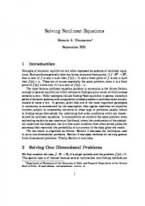
We have been provided with a simplified version of the AProVE tool, which is parameterized by the solver. The system is also based on the dependency pair method and generates polynomial constraints over the integers and the rational numbers. As before, the constraints are sent to the solver which in turn returns a solution if one is found. BOUND 1 BOUND 2 SAT HySAT SMT SAT HySAT SMT Total Time Total Time Total Time Total Time Total Time Total Time YES 649 864 649 783 649 790 701 1360 697 1039 701 1191 MAYBE 1093 2289 1091 2259 1093 2233 1039 2449 1033 2818 1033 2225 KILLED 13 15 13 15 25 21 BOUND 4 BOUND 7 SAT HySAT SMT SAT HySAT SMT Total Time Total Time Total Time Total Time Total Time Total Time YES 705 1596 705 1446 710 1222 705 1762 702 1246 708 1357 MAYBE 1014 3551 967 4061 1019 2481 989 4224 871 4482 1008 2862 KILLED 36 83 26 61 182 39 Fig. 2. Experiments with integers in AProVE

In order to check not only the performance of our solver compared to the AProVE original one, but also with some other existing solver for non-linear arithmetic, we have included, in the case of integer domains, a comparison with HySAT, a solver for non-linear arithmetic based on interval analysis. Although HySAT can give, in general, wrong solutions (as said in its own documentation), it has never happened to us when considering integers. Moreover, in the case of integers, the comparison is completely fair since we send to HySAT exactly the same constraint provided by AProVE adding only the declaration of the variables with the integer interval under consideration (for instance, int [0,4] x). We have included here the results using HySAT since all three solvers can handle the same domains. The results in Figure 2 show that, in general, HySAT is a little faster when the answer is YES, but has a lot more KILLED problems. On the other hand, our solver is in general faster than the SAT-based AProVE solver and always

faster in the overall runtime (without counting timeouts), starting very similar and increasing as the domain grows. This improvement is more significant if we take into account that there is an important part of the process that is common (namely the generation of constraints) independently of the solver. Moreover, the number of KILLED problems by our solver is only bigger than or equal to that of the SAT-based one for the smallest two domains but is always the lowest from that point on and the difference grows as the domain is enlarged. 0..16/4

SAT HySAT SMT Total Time Total Time Total Time YES 797 3091 774 2088 824 2051 MAYBE 666 6605 508 3078 826 4380 KILLED 292 473 105

SMT

Q4 Q4+8 Total Time Total Time YES 833 1755 834 1867 MAYBE 876 2861 870 2910 KILLED 46 51

Fig. 3. Experiments with rationals in AProVE

Regarding the use of rationals, we can only compare the performance on domains of rationals as integers with fixed denominator and a bounded numerator, since this is the only case the original solver of our version of AProVE can handle (more general domains are available in the full version of AProVE, but they turned out to have a poorer performance). In particular, we have considered the domain 0..16/4. Additionally, we have included the results of AProVE when using our solver on the domain Q4 and Q4 + 8 since these are the domains which overall produce the best results in number of YES. As for integer intervals, Figure 3 shows that our solver has a better performance, when comparable, than the other two solvers when using rationals. Moreover, we obtain the best overall results when using our solver with rational domains that are not handled by any other solver.

4

Conclusions

We have proposed a simple method for solving non-linear polynomial constraints over finite domains of the integer and the rational numbers, which is based on translating the constraints into SAT modulo linear (real or integer) arithmetic. Our method can handle general boolean formulas and domains with negative values for free, making them available for future improvements in termination tools. By means of several experiments, our solvers are shown to be faster and more flexible in handling different solution domains than all their predecessors. Altogether, we believe that these results can have both an immediate and a future impact on termination tools. As future work, we want to analyze the usefulness of some features that the SMT solvers usually have, like being incremental or backtrackable, to avoid repeated work when proving termination of a TRS. Acknowledgments: we would like to thank J¨ urgen Giesl, Carsten Fuhs and Karsten Behrmann for their very quick reaction in providing us with a version of AProVE to be used in our experiments, and especially to Carsten for some interesting and helpful discussion on possible useful extensions of the solver.

References 1. T. Arts and J. Giesl. Termination of Term Rewriting Using Dependency Pairs. Theoretical Computer Science, 236:133-178, 2000. 2. S. Basu, R. Pollack and M.-F. Roy. Algorithms in Real Algebraic Geometry. Springer-Verlag, 2003. 3. M. Bofill, R. Nieuwenhuis, A. Oliveras, E. Rodr´ıguez-Carbonella and A. Rubio. The Barcelogic SMT Solver. Proc. of 20th CAV, LNCS 5123, 2008. 4. E. Contejean and C. March´e, B. Monate and X. Urbain. Proving termination of rewriting with CiME. Proc. of 6th Int. Workshop on Termination, 2003. 5. E. Contejean, C. March´e, A.-P. Tom´ as, and X. Urbain. Mechanically proving termination using polynomial interpretations. Journal of Automated Reasoning, 34(4):325-363, 2006. 6. B. Dutertre and L. de Moura. The Yices SMT solver. System description report. http://yices.csl.sri.com/ 7. B. Dutertre and L. de Moura. A Fast Linear-Arithmetic Solver for DPLL(T). Proc. of 18th CAV, LNCS 4144, 2006. 8. M. Fr¨ anzle, C. Herde, T. Teige, S. Ratschan, and T. Schubert. Efficient Solving of Large Non-linear Arithmetic Constraint Systems with Complex Boolean Structure. Journal on Satisfiability, Boolean Modeling and Computation 1:209-236, 2007. 9. C. Fuhs, J. Giesl, A. Middeldorp, P. Schneider-Kamp, R. Thiemann, H. Zankl Maximal Termination. Proc. of 19th RTA, LNCS 5117, 2008. 10. C. Fuhs, J. Giesl, A. Middeldorp, P. Schneider-Kamp, R. Thiemann, and H. Zankl. SAT Solving for Termination Analysis with Polynomial Interpretations. Proc. of 10th SAT, LNCS 4501, 2007. 11. C. Fuhs, R. Navarro-Marset, C. Otto, J. Giesl, S. Lucas, and P. Schneider-Kamp. Search Techniques for Rational Polynomial Orders. In Proc. of 9th AISC, Springer LNAI 5144, 2008. 12. J. Giesl. Generating Polynomial Orderings for Termination Proofs. In Proc. of 6th RTA, LNCS 914, 1995. 13. J. Giesl, P. Schneider-Kamp, and R. Thiemann. AProVE 1.2: Automatic Termination Proofs in the Dependency Pair Framework. 3rd Int. Joint Conference on Automated Reasoning , LNAI 4130, 2006. 14. S. Gulwani and A. Tiwari. Constraint-Based Approach for Analysis of Hybrid Systems Proc. of 20th CAV, LNCS 5123, 2008. 15. N. Hirokawa and A. Middeldorp. Polynomial Interpretations with Negative Coefficients. In Proc. of AISC’04, Springer LNAI 3249, 2004. 16. N. Hirokawa and A. Middeldorp. Tyrolean termination tool: Techniques and features. Information and Computation, 205:474-511, 2007. 17. S. Lucas. MU-TERM: A Tool for Proving Termination of Context-Sensitive Rewriting. In Proc. of RTA’04, LNCS 3091, 2004. http://zenon.dsic.upv.es/muterm. 18. S. Lucas. Polynomials over the reals in proofs of termination: from theory to practice. RAIRO Theoretical Informatics and Applications, 39(3):547-586, 2005. 19. S. Lucas. Practical use of polynomials over the reals in proofs of termination. Proc. of 9th PPDP, ACM Press, 2007. 20. L. de Moura and N. Bjorner. Z3: An Efficient SMT Solver. Proc. of 14th TACAS, LNCS 4963, 2008. 21. M.T. Nguyen and D. De Schreye. Polynomial Interpretations as a Basis for Termination Analysis of Logic Programs. In Proc. of 21st ICLP, LNCS 3668, 2005.