Solving Singular Boundary Value Problems by Optimal Homotopy

Hindawi Publishing Corporation International Journal of Diﬀerential Equations Volume 2014, Article ID 287480, 10 pages http://dx.doi.org/10.1155/2014/287480

Research Article Solving Singular Boundary Value Problems by Optimal Homotopy Asymptotic Method S. Zuhra,1 S. Islam,2 M. Idrees,2 Rashid Nawaz,1,2 I. A. Shah,2 and H. Ullah1 1 2

Department of Mathematics, Islamia College University Peshawar, Pakistan Department of Mathematics, Abdul Wali Khan University, Mardan, Khyber Pakhtunkhwa, Pakistan

Correspondence should be addressed to H. Ullah; [email protected] Received 14 February 2014; Revised 1 June 2014; Accepted 2 June 2014; Published 29 June 2014 Academic Editor: Domiri D. Ganji Copyright © 2014 S. Zuhra et al. This is an open access article distributed under the Creative Commons Attribution License, which permits unrestricted use, distribution, and reproduction in any medium, provided the original work is properly cited. In this paper, optimal homotopy asymptotic method (OHAM) for the semianalytic solutions of nonlinear singular two-point boundary value problems has been applied to several problems. The solutions obtained by OHAM have been compared with the solutions of another method named as modified adomain decomposition (MADM). For testing the success of OHAM, both of the techniques have been analyzed against the exact solutions in all problems. It is proved by this paper that solutions of OHAM converge rapidly to the exact solution and show most effectiveness as compared to MADM.

1. Introduction Nonlinear singular boundary values problem (SBVP) is of considerable importance in the modeling of many branches of mathematical physics and engineering i-e fluid mechanics, quantum mechanics, astrophysics and so forth. Nonlinear problems are difficult to solve as compared to linear problems but the singularity of such nonlinear problem becomes more difficult to solve by researcher. Such type of problems have been successfully solved by modified adomian decomposition method [1, 2], but the convergence rate of its series goes gradually to accurate solution. Recently a new growing method has been introduced by Marinca et al. [3–6], for approximate solution of the problems of thin film flow of a fourth grade fluid on a cylinder surface and for understanding the behavior of nonlinear mechanical vibration of an electrical machines. OHAM attracted great attention of many researchers to solve a large class of linear and nonlinear differential equations and so forth; Idrees et al. extended OHAM by applying on initial and boundary values problems of ODEs and PDEs [7–10]. Iqbal and Javed [11] applied OHAM for the analytical solution of singular Lane-Emden type equations. The goal of this paper is to apply the proposed method to compute best approximate solutions of nonlinear singular boundary values problems. This paper is arranged

in four sections; the first section of the paper describes the introduction, the second section of the paper is about the basic idea of OHAM, and the third section presents numerical results to demonstrate the efficiency of OHAM, and the last section of the paper is the conclusion.

2. Basic Mathematical Theory of Optimal Homotopy Asymptotic Method The framework of OHAM is given in few steps. (i) Consider the undertaken differential equation L (𝑤 (𝜉, 𝜏)) + N (𝑤 (𝜉, 𝜏)) + g (𝜉, 𝜏) = 0, B (𝑤, 𝑤𝜏 ) = 0,

(1)

where 𝜉 and 𝜏 are independent variables and L(𝑤(𝜉, 𝜏)) and N(𝑤(𝜉, 𝜏)) are linear and nonlinear part of (1), respectively. Simply linear operator is denoted by L and nonlinear by N, 𝑤(𝜉, 𝜏) is taken as an unknown function, g(𝑥, 𝜏) is considered as known function, and B(𝑤, 𝑤𝜏 ) yield corresponding initial condition. Now

2

International Journal of Differential Equations

(ii) According to OHAM, an optimal homotopy, 𝜑(𝜉, 𝑞) : B × [0, 1] → 𝑅 can be built, fulfilling homotopy equation: (1 − 𝑑) [L (𝜑 (𝜉, 𝜏; 𝑑)) + g (𝜉, 𝜏)] = H (𝑑) [L (𝜑 (𝜉, 𝜏; 𝑑)) + g (𝜉, 𝜏) + N (𝜑 (𝜉, 𝜏; 𝑑))] ,

L (𝑤2 (𝜉, 𝜏)) − L (𝑤1 (𝜉, 𝜏)) { { { { { = 𝐾2 N0 (𝑤0 (𝜉, 𝜏)) { { { +𝐾1 (L (𝑤1 (𝜉, 𝜏)) + N1 (𝑤0 (𝜉, 𝜏)) , 𝑤1 (𝜉, 𝜏)) , { { { { { { { { B (𝑤2 , 𝑑𝑤2 ) = 0 𝑑𝜉 {

B (𝜑 (𝜉, 𝜏; 𝑑)) = 0,

.. .

(2) H(𝑑) is auxiliary function with 𝑑 ∈ [0, 1], an embedding parameter, such that ∞

{ {∑ 𝐾𝑗 𝑑𝑗 , H (𝑑) = {𝑗=1 { {0,

𝑑 ≠ 0,

(3)

𝑑 = 0.

𝑑 varies from 0 to 1 and the solution 𝜑(𝜉, 𝜏; 𝑑) varies from 𝑤0 (𝜉, 𝜏) to the final solution 𝑤(𝜉, 𝜏), where 𝑤0 (𝜉, 𝜏) is evaluated from (2) for 𝑑 = 0: B (𝑤0 , 𝑤𝜉 ) = 0.

L (𝑤0 (𝜉, 𝜏)) + g (𝜉, 𝜏) = 0,

(4)

H(𝑑) is reserved in the series as below: H (𝑑) = 𝑑𝐾1 + 𝑑2 𝐾2 + 𝑑3 𝐾3 + ⋅ ⋅ ⋅ .

(5)

(iii) Next 𝜑(𝜉, 𝜏; 𝑑 : 𝐾𝑖 ) can be spread out by Taylor’s series about the parameter 𝑑: 𝜑 (𝜉, 𝜏; 𝑑 : 𝐾𝑖 ) = 𝑤0 (𝜉, 𝜏) + ∑ 𝑤𝑘 (𝜉, 𝜏; 𝐾𝑖 ) 𝑑𝑘 , 𝑘≥1

(6)

𝑖 = 1, 2, . . . . 𝐾1 , 𝐾2 , . . ., cause the accurateness and convergence of (6) and if it converges at 𝑑 = 1 then we have the following (see [5]):

L (𝑤𝑘 (𝜉, 𝜏)) − L (𝑤𝑘−1 (𝜉, 𝜏)) } { } { } { } { } { = 𝐾 N (𝑤 𝜏)) (𝜉, } { 𝑘 0 0 } { } { } { } { 𝑘−1 } { } { } { 𝜏)) 𝐾 (L (𝑤 + ∑ (𝜉, } { 𝑖 𝑘−1 } { } { 𝑖=1 } { } { +N𝑘−1 (𝑤0 (𝜉, 𝜏) , } { } { } { } { } { } { } { 𝜏) , . . . , 𝑤 𝜏))) , 𝑤 (𝜉, (𝜉, } { 1 𝑘−𝑖 } { } { } { } { 𝑑𝑤 } { 𝑘 } { B (𝑤𝑘 , )=0 𝑑𝜉 } { 𝑘 = 2, 3, 4, . . . . (10) (iv) The resultant linear problems can now be solved and their solutions are used to construct 𝐾th order solution that comprises 𝐾𝑖 of the original problem through (7). Then by substituting (7) into (1), we get the following residual: 𝑅 (𝜉, 𝜏; 𝐾𝑖 ) = L (̃ 𝑤(𝑚) (𝜉, 𝜏; 𝐾𝑖 )) + g (𝜉, 𝜏) + N (̃ 𝑤(𝑚) (𝜉, 𝜏; 𝐾𝑖 )) ,

𝜑 (𝜉, 𝜏; 𝐾𝑖 ) = 𝑤0 (𝜉, 𝜏) + ∑ 𝑤𝑘 (𝜉, 𝜏; 𝐾𝑖 ) 𝑑𝑘 ,

𝑖 = 1, 2, . . . , 𝑚.

(11)

when 𝑅(𝜉, 𝜏; 𝐾𝑖 ) = 0, for some values of 𝐾𝑖 then L(̃ 𝑤(𝑚) (𝜉, 𝜏; 𝐾𝑖 )) will agree with the exact solution. Though, this does not occur generally, especially, in nonlinear problems. Therefore, optimal values of the auxiliary constants 𝐾1 , 𝐾2 , . . . , 𝐾𝑛 are calculated for minimizing the following functional 𝐽 (see [5]): 1

𝑚

} } } } } } } } } } } } } } } } } (9)

𝐽 (𝐾1 , 𝐾2 , . . . , 𝐾𝑛 ) = ∫ 𝑅2 (𝜉, 𝐾1 , 𝐾2 , . . . , 𝐾𝑚 ) 𝑑𝜉. 0

(12)

k=1

(7) Insert (6) into homotopy formula (2) and comparing like powers of 𝑑, the original nonlinear problem transferred into a sequence of linear problems, we obtained zeroth order (4), first order (8), second order (9), and 𝐾th order (10) as below: L (𝑤1 (𝜉, 𝜏)) = 𝐾1 N0 (𝑤0 (𝜉, 𝜏)) ,

B (𝑤1 ,

𝑑𝑤1 ) = 0, 𝑑𝜉 (8)

Therefore, the unknown constants 𝐾𝑖 (𝑖 = 1, 2, . . . 𝑚) can be optimally identified from the following conditions (see [5]): 𝜕𝐽 𝜕𝐽 𝜕𝐽 = = ⋅⋅⋅ = = 0. 𝜕𝐾1 𝜕𝐾2 𝜕𝐾𝑚

(13)

With these known values of the auxiliary constants the approximate solution (7) is now well determined.


3

3. Application of OHAM

Its solution is

OHAM is implemented on three models of singular boundary value problems in order to show the accuracy of this method.

𝑤1 (𝜉, 𝐾1 , 𝐾2 ) = 𝐾1 (0.0637828𝜉2 − 0.0416667𝜉4 + 0.00751757𝜉6 − 0.000813799𝜉8 + 0.0000528577𝜉10

Model 3.1. Consider second order singular boundary value problem [1]:

−1.90734 × 10−6 𝜉12 + 2.94964 × 10−8 𝜉14 )

2

1 𝜉 𝑤󸀠󸀠 (𝜉) − 𝑤󸀠 (𝜉) = 𝑤5 (𝜉) , 𝜉 3

(14)

+ 𝐾12 (0.0700404𝜉2 − 0.0416667𝜉4 + 0.00308821𝜉6

subject to boundary conditions 𝑤 (0) = 1,

𝑤󸀠 (1) = −0.216506

+ 0.00159194𝜉8 − 0.000573068𝜉10 (15)

+ 0.0000997917𝜉12 − 0.000011419𝜉14

with exact solution 𝑤 (𝜉) = (1 +

2

+ 9.36638 × 10−7 𝜉16

−1/2

𝜉 ) 3

.

(16)

− 5.633 × 10−8 𝜉18 + 2.43915 × 10−9 𝜉20 − 7.20125 × 10−11 𝜉22

Zeroth Order Problem. Consider the following: 𝑤0󸀠󸀠 (𝑥) = 𝑤0 (0) = 1,

𝑤0󸀠

𝑤0󸀠 (𝜉) , 𝜉

+1.29926 × 10−12 𝜉24 − 1.08191 × 10−14 𝜉26 ) (17)

+ 𝐾2 (0.0637828𝜉2 − 0.0416667𝜉4 + 0.00751757𝜉6

(1) = −0.216506.

− 0.000813799𝜉8 + 0.0000528577𝜉10

Its solution is 𝑤0 (𝜉) = 1 − 0.108253𝜉2 .

−1.90734 × 10−6 𝜉12 + 2.94964 × 10−8 𝜉14 ) . (22)

(18)

First Order Problem. Consider the following: 𝑤1󸀠󸀠 (𝜉) − 𝑤0󸀠󸀠 (𝜉) (1 + 𝐾1 ) −

+ 0.3333333𝜉2 𝐾1 𝑤05 (𝜉) = 0, 𝑤1 (0) = 0,

Solve (17) to (22) to obtain approximate solution in the form of

𝑤1󸀠 (𝜉) 𝑤0󸀠 (𝜉) + (1 + 𝐾1 ) 𝜉 𝜉

𝑤1󸀠

(19)

(1) = 0.

̃ (𝜉, 𝐾1 , 𝐾2 ) = 𝑤0 (𝜉) + 𝑤1 (𝜉, 𝐾1 ) + 𝑤2 (𝜉, 𝐾1 , 𝐾2 ) . 𝑤

(23)

To determine constant values, 𝐾1 and 𝐾2 , apply the method of least square (12), (13) where

Its solution is 𝑤1 (𝜉, 𝐾1 )

𝐾1 = −0.902176342508146,

(24)

= (0.0637828𝜉2 − 0.0416667𝜉4 + 0.00751757𝜉6

𝐾2 = −0.004742918346272.

− 0.000813799𝜉8 + 0.0000528577𝜉10

By substituting values of 𝐾1 and 𝐾2 in (22), we achieved the approximate solution of OHAM.

−1.90734 × 10−6 𝜉12 + 2.94964 × 10−8 𝜉14 ) 𝐾1 . (20)

Model 3.2. Consider the following third order nonlinear boundary value problem [2]:

Second Order Problem. Consider the following: 𝑤󸀠󸀠󸀠 (𝜉) −

𝑤2󸀠󸀠 (𝜉) − 𝑤1󸀠󸀠 (𝜉) (1 + 𝐾1 ) − 𝐾2 𝑤0󸀠󸀠 (𝜉) −

𝐾 𝑤󸀠 (𝜉) 𝑤2󸀠 (𝜉) 𝑤1󸀠 (𝜉) + (1 + 𝐾1 ) + 2 0 𝜉 𝜉 𝜉

+ 0.3333333𝜉2 𝐾2 𝑤05 (𝜉) + 1.6666667𝜉2 𝐾1 𝑤04 (𝜉) 𝑤1 (𝜉) = 0, 𝑤2 (0) = 0,

𝑤2󸀠 (1) = 0.

2 󸀠󸀠 𝑤 (𝜉) − 𝑤 (𝜉) − 𝑤2 (𝜉) = ℎ (𝜉) , 𝑥

(25)

with boundary conditions (21)

𝑤 (0) = 0,

𝑤󸀠 (0) = 0,

𝑤 (1) = 2.71828182, (26)

where ℎ (𝜉) = 7𝜉2 𝑒𝜉 + 6𝜉𝑒𝜉 − 6𝑒𝜉 − 𝜉6 𝑒2𝜉 .

(27)

4

International Journal of Differential Equations + 2.60148 × 10−9 𝜉23 − 1.57505 × 10−9 𝜉24

Zeroth Order Problem. Consider the following:

− 1.38639 × 10−9 𝜉25 − 6.93534 × 10−10 𝜉26

2𝑤0󸀠󸀠 (𝜉) 17 41 2 𝑤0󸀠󸀠󸀠 (𝜉) = − 6 + 10𝜉2 + 9𝜉3 + 𝜉4 + 𝜉5 − 𝜉6 𝜉 4 30 3 325 7 5729 8 20137 9 67181 10 − 𝜉 − 𝜉 − 𝜉 − 𝜉 , 168 2880 15120 100800 𝑤0󸀠

𝑤0 (0) = 0,

(0) = 0,

𝑤0 (1) = 2.71828182. (28)

Its solution is

9

+ 0.00610119𝜉 − 0.00185185𝜉 − 0.00358245𝜉

10

− 0.00258342𝜉11 − 0.00126119𝜉12 − 0.0004747𝜉13 . (29) First Order Problem. Consider the following: 𝑤1󸀠󸀠󸀠 (𝜉) − 𝑤0󸀠󸀠󸀠 (𝜉) (1 + 𝐾1 ) −

2𝑤1󸀠󸀠 (𝜉) 2𝑤0󸀠󸀠 (𝜉) + (1 + 𝐾1 ) 𝜉 𝜉

17 41 2 325 7 + (−6 + 10𝜉 + 9𝜉 + 𝜉4 + 𝜉5 − 𝜉6 − 𝜉 4 30 3 168 5729 8 20137 9 67181 10 − 𝜉 − 𝜉 − 𝜉 ) (1 + 𝐾1 ) = 0, 2880 15120 100800 3

𝑤1󸀠 (0) = 0,

𝑤1 (0) = 0,

(31) Second Order Problem. Consider the following: 𝜉𝑦2󸀠󸀠󸀠 (𝑥) − 𝜉𝐾1 𝑦1󸀠󸀠󸀠 (𝜉) − 𝜉𝑦1󸀠󸀠󸀠 (𝜉) − 𝜉𝐶2 𝑦0󸀠󸀠󸀠 (𝜉) + 2𝐾1 𝑦1󸀠󸀠 (𝜉)

+ 𝜉𝐾2 𝑦02 (𝜉) + 𝜉𝐾2 𝑦0 (𝜉) − 2𝑦2󸀠󸀠 (𝜉) + 2𝑦1󸀠󸀠 (𝜉) − 6𝜉𝐾2 + 10𝜉3 𝐾2 + 9𝜉4 𝐾2 +

𝑤1 (1) = 0. (30)

Its solution is

17 5 41 𝜉 𝐾2 + 𝜉6 𝐾2 4 30

2 325 8 5729 9 − 𝜉7 𝐾2 − 𝜉 𝐾2 − 𝜉 𝐾2 3 168 2880 −

+ 𝑤02 (𝜉) 𝐾1 + 𝑤0 (𝜉) 𝐾1 2

−1.11005 × 10−11 𝜉29 ) .

+ 2𝐾2 𝑦0󸀠󸀠 (𝜉) + 2𝜉𝐾1 𝑦0 (𝜉) 𝑦1 (𝜉) + 𝜉𝐾1 𝑦1 (𝜉)

𝑤0 (𝜉) = 𝜉3 + 1.0382𝜉4 + 0.5𝜉5 + 0.15𝜉6 + 0.0337302𝜉7 8

− 2.50421 × 10−10 𝜉27 − 6.59925 × 10−11 𝜉28

20137 10 67181 11 𝜉 𝐾2 − 𝜉 𝐾2 = 0, 15120 100800 𝑤2 (0) = 0,

𝑤2󸀠 (0) = 0,

𝑤2 (1) = 0. (32)

Its solution is 𝑤2 (𝜉, 𝐾1 , 𝐾2 ) = 7.544 × 10−18 𝜉4 − 7.04904 × 10−18 𝜉7 − 9.91271 × 10−19 𝜉8 − 3.08395 × 10−19 𝜉9 + 4.11194 × 10−19 𝜉10 + 2.8837 × 10−19 𝜉11 + 1.05135 × 10−19 𝜉12 + 1.05135 × 10−19 𝜉13

𝑤1 (𝜉, 𝐾1 ) −18 4

= 7.544 × 10

𝜉 − 7.04904 × 10 −19 8

− 9.91271 × 10

+ 𝐾1 (0.0388054𝜉4 − 0.0166667𝜉6

−18 7

𝜉

− 0.00823971𝜉7 − 0.00223214𝜉8 − 0.00319444𝜉9

−19 9

𝜉 − 3.08395 × 10

𝜉

+ 4.11194 × 10−19 𝜉10 + 2.8837 × 10−19 𝜉11 + 1.05135 × 10−19 𝜉12 + 𝐾1 (0.0388054𝜉4 − 0.0166667𝜉6 − 0.00823971𝜉7

− 0.00390766𝜉10 − 0.00270645𝜉11 − 0.00126549𝜉12 − 0.000445398𝜉13 − 0.000126185𝜉14 − 0.000027677𝜉15

− 0.00223214𝜉8 − 0.00319444𝜉9

− 1.64425 × 10−6 𝜉16 + 3.24922 × 10−6 𝜉16

− 0.00390766𝜉10 − 0.00270645𝜉11

+ 2.71079 × 10−6 𝜉18 + 1.42573 × 10−6 𝜉19

− 0.00126549𝜉12 − 0.000445398𝜉13 14

15

− 0.000126185𝜉 − 0.000027677𝜉 −6 16

− 1.64425 × 10 𝜉

+ 3.24922 × 10−6 𝜉16 + 2.71079 × 10−6 𝜉18

+ 5.40486 × 107 𝜉20 + 1.49526 × 10−7 𝜉21 + 2.95509 × 10−8 𝜉22 + 2.60148 × 10−9 𝜉23 − 1.57505 × 10−9 𝜉24 − 1.38639 × 10−9 𝜉25

+ 1.42573 × 10−6 𝜉19 + 5.40486 × 107 𝜉20

− 6.93534 × 10−10 𝜉26 − 2.50421 × 10−10 𝜉27

+ 1.49526 × 10−7 𝜉21 + 2.95509 × 10−8 𝜉22

−6.59925 × 10−11 𝜉28 − 1.11005 × 10−11 𝜉29 )


5

+ 𝐾12 (0.03692188𝜉4 − 0.0166667𝜉6

− 1.86591 × 10−16 𝜉40 − 8.03133 × 10−17 𝜉41

− 0.00854769𝜉7 − 0.00223214𝜉8

− 2.61417 × 10−17 𝜉42 − 6.5531 × 10−18 𝜉43

− 0.0031481510𝜉9 − 0.00403613𝜉10

−1.19784 × 10−18 𝜉44 − 1.2982 × 10−19 𝜉45 )

− 0.0028082𝜉11 − 0.00126764𝜉12

+ 𝐾2 (0.0388054𝜉4 − 0.0166667𝜉6

− 0.00041452𝜉13 − 0.000105125𝜉14 × 10−6 𝜉16

− 0.00823971𝜉7 − 0.00223214𝜉8

+ 8.49649 × 10−6 𝜉17 + 5.8467 × 10−6 𝜉18

− 0.00319444𝜉9 − 0.00390766𝜉10

+ 2.90517 × 10−6 𝜉19 + 1.10585 × 10−6 𝜉20

− 0.00270645𝜉11 − 0.00126549𝜉12

+ 3.2565 × 10−7 𝜉21 + 7.18826 × 10−8 𝜉22

− 0.000445398𝜉13 − 0.000126185𝜉14

+ 6.70135 × 10−9 𝜉23 − 5.45808 × 10−9 𝜉24

− 0.000027677𝜉15 − 1.64425 × 10−6 𝜉16

− 4.99343 × 10−9 𝜉25 − 2.6526 × 10−9 𝜉26

+ 3.24922 × 10−6 𝜉16 + 2.71079 × 10−6 𝜉18

− 1.05107 × 10−9 𝜉27 − 3.27247 × 10−10 𝜉28

+ 1.42573 × 10−6 𝜉19 + 5.40486 × 107 𝜉20

+ 7.96076 × 10−11 𝜉29 − 1.3044 × 10−11 𝜉30

+ 1.49526 × 10−7 𝜉21 + 2.95509 × 10−8 𝜉22

− 4.36977 × 10−13 𝜉31 − 1.22809 × 10−12 𝜉32

+ 2.60148 × 10−9 𝜉23 − 1.57505 × 10−9 𝜉24

+ 8.15668 × 10−13 𝜉33 + 3.55887 × 10−13 𝜉34

− 1.38639 × 10−9 𝜉25 − 6.93534 × 10−10 𝜉26

+ 1.20393 × 10−13 𝜉35 + 3.18368 × 10−14 𝜉36

− 2.50421 × 10−10 𝜉27 − 6.59925 × 10−11 𝜉28

+ 6.13738 × 10−15 𝜉37 + 5.19104 × 10−16 𝜉38

−1.11005 × 10−11 𝜉29 ) .

− 2.50795 × 10−16 𝜉39 − 1.86591 × 10−16 𝜉40 − 8.03133 × 10−17 𝜉41 − 2.61417 × 10−17 𝜉42 − 6.5531 × 10−18 𝜉43 − 1.19784 × 10−18 𝜉44 −19 45

− 1.2982 × 10

(33) Solving problem (28) to (33), in the form of ̃ (𝜉, 𝐾1 , 𝐾2 ) = 𝑤0 (𝜉) + 𝑤1 (𝜉, 𝐾1 ) + 𝑤2 (𝜉, 𝐾1 , 𝐾2 ) . 𝑤

15

𝜉 − 0.0000168305𝜉

+ 5.60083 × 10−6 𝜉16 + 8.49649 × 10−6 𝜉17

We obtained the constant values of 𝐾1 and 𝐾2 as 𝐾1 = −0.615104986973096,

+ 5.8467 × 10−6 𝜉18 + 2.90517 × 10−6 𝜉19

𝐾2 = −0.11776184847135589.

+ 1.10585 × 10−6 𝜉20 + 3.2565 × 10−7 𝜉21 −8 22

−9 23

+ 7.18826 × 10 𝜉 + 6.70135 × 10 𝜉

− 5.45808 × 10−9 𝜉24 − 4.99343 × 10−9 𝜉25 − 2.6526 × 10−9 𝜉26 − 1.05107 × 10−9 𝜉27 − 3.27247 × 10−10 𝜉28 + 7.96076 × 10−11 𝜉29 − 1.3044 × 10−11 𝜉30 − 4.36977 × 10−13 𝜉31

+ 3.55887 × 10

𝑤 (𝜉) = 𝜉3 + 𝜉4 + 0.5𝜉5 + 0.166666𝜉6 + 0.04166666𝜉7 + 0.008333𝜉8 + 0.0013888𝜉9 + 0.000198𝜉10 + ⋅ ⋅ ⋅ . (36) Model 3.3. Consider the following third order singular boundary value problem [1]: 2 𝑤󸀠󸀠󸀠 (𝜉) − 𝑤󸀠󸀠 (𝜉) − 𝑤3 (𝜉) = ℎ (𝜉) , 𝜉

−13 35

𝜉 + 1.20393 × 10

𝜉

+ 3.18368 × 10−14 𝜉36 + 6.13738 × 10−15 𝜉37 + 5.19104 × 10−16 𝜉38 − 2.50795 × 10−16 𝜉39

(35)

Taylor series of the exact solution with order 10, which is given below

− 1.22809 × 10−12 𝜉32 + 8.15668 × 10−13 𝜉33 −13 34

(34)

(37)

subject to boundary conditions 𝑤 (0) = 0,

𝑤󸀠 (0) = 0,

𝑤󸀠 (1) = 10.8371,

(38)

6

International Journal of Differential Equations + 𝐾1 (2.96059 × 10−16 𝜉3 + 0.0348465𝜉4

where ℎ (𝜉) = 7𝜉2 𝑒𝜉 + 6𝜉𝑒𝜉 − 6𝑒𝜉 − 𝑥9 𝑒3𝜉 + 𝑥3 𝑒𝜉 .

− 7.04904 × 10−18 𝜉7 − 1.98254 × 10−18 𝜉8

(39)

Exact solution of (41) is

+ 2.56996 × 10−20 𝜉10 + 9.01155 × 10−21 𝜉11

3 𝜉

𝑤 (𝜉) = 𝜉 𝑒 .

(40)

− 0.00094697𝜉12 − 0.00215765𝜉13

Zeroth Order Problem. Consider the following: 𝑤0󸀠󸀠󸀠 (𝜉) −

2𝑤0󸀠󸀠

(𝜉)

𝜉

− 0.000250492𝜉14 − 0.00197358𝜉15

+ 6 − 10𝜉2 − 10𝜉3 − 5.25𝜉4

− 0.00118551𝜉16 − 0.000578225𝜉17

− 1.86666666667𝜉5 − 0.5𝜉6 − 0.107142857143𝜉7

− 0.000238163𝜉18 − 0.0000850952𝜉19

− 0.0190972222224𝜉8 + 0.9970899470899471𝜉9

− 0.0000268863𝜉20 − 7.225 × 10−6 𝜉21

+ 2.9996130952380953𝜉10 = 0,

− 5.00972 × 10−7 𝜉22 (41)

𝑤0󸀠 (0) = 0,

𝑤0 (0) = 0,

𝑤0󸀠 (1) = 10.8731.

+ 1.4809 × 10−6 𝜉23 + 1.41769 × 10−6 𝜉24

(42)

+ 8.1403 × 10−7 𝜉25 + 3.49615 × 10−7 𝜉26

Its solution is

+ 1.21188 × 10−7 𝜉27 + 3.53307 × 10−8 𝜉28

𝑤0 (𝜉) = 𝜉3 + 1.0097𝜉4 + 0.5𝜉5 + 0.166667𝜉6

+ 8.89992 × 10−9 𝜉29 + 1.85617 × 10−9 𝜉30

+ 0.0416667𝜉7 + 0.00833333𝜉8 + 0.00138889𝜉9

− 1.99788 × 10−10 𝜉31 − 9.12587 × 10−10 𝜉32

+ 0.000198413𝜉10 + 0.0000248016𝜉11

− 6.52991 × 10−10 𝜉33 − 2.65181 × 10−10 𝜉34

− 0.000944214𝜉12 − 0.00213648𝜉13 .

− 7.59661 × 10−11 𝜉35 − 1.67268 × 10−11 𝜉36

(43)

− 2.98912 × 10−12 𝜉37 − 4.49394 × 10−13 𝜉38

First Order Problem. Consider the following: 𝑤1󸀠󸀠󸀠 (𝜉) − 𝑤0󸀠󸀠󸀠 (𝜉) (1 + 𝐾1 ) − +

2𝑤0󸀠󸀠

𝜉

(𝜉)

2𝑤1󸀠󸀠 (𝜉) 𝜉

− 4.19389 × 10−14 𝜉39 + 9.57023 × 10−14 𝜉40 +2.1308 × 10−13 𝜉41 + 1.49031 × 10−13 𝜉42 ) .

(1 + 𝐾1 ) + 𝑤02 (𝜉) 𝐾1

(45)

− (6 − 10𝜉2 − 9𝜉3 − 5.25𝜉4

Second Order Problem. Consider the following:

− 1.86666666667𝜉5 − 0.5𝜉6 − 0.107142857143𝜉7 − 0.0190972222224𝜉8 + 0.9970899470899471𝜉9 +2.9996130952380953𝜉10 ) (1 + 𝐾1 ) = 0, 𝑤1 (0) = 0,

𝑤1󸀠 (0) = 0,

𝑤1󸀠 (1) = 0.

Its solution is 𝑤1 (𝜉, 𝐾1 ) = 2.96059 × 10−16 𝜉3 − 2.07889 × 10−16 𝜉4 − 7.04904 × 10−18 𝜉7 − 1.98254 × 10−18 𝜉8 + 2.56996 × 10−20 𝜉10 + 9.01155 × 10−21 𝜉11 + 6.32606 × 10−19 𝜉13

𝑤2󸀠󸀠󸀠 (𝜉) − 𝑤1󸀠󸀠󸀠 (𝜉) (1 + 𝐾1 ) − 𝑤0󸀠󸀠󸀠 (𝜉) 𝐾2 −

2𝐾2 𝑤0󸀠󸀠 (𝜉) 2𝑤2󸀠󸀠 (𝜉) 2𝑤1󸀠󸀠 (𝜉) + (1 + 𝐾1 ) + 𝜉 𝜉 𝜉

+ 3𝐾1 𝑤02 (𝜉) 𝑤1 (𝜉) + 𝐾2 𝑤03 (𝜉) − 𝑤1󸀠󸀠󸀠 (𝜉) (44)

− 𝑤0󸀠󸀠󸀠 (𝜉) (1 + 𝐾1 ) − (6 − 10𝜉2 − 10𝜉3 − 5.25𝜉4 − 1.86666666667𝜉5 − 0.5𝜉6 − 0.107142857143𝜉7 − 0.0190972222224𝜉8 + 0.9970899470899471𝜉9 +2.9996130952380953𝜉10 ) 𝐾2 = 0, 𝑤2 (0) = 0,

𝑤2󸀠 (0) = 0,

𝑤2󸀠 (1) = 0.

(46)


7

Table 1: Comparison of second order OHAM solution with exact solution and third order MADM solution up to order 14. 𝜉 0.1 0.2 0.3 0.4 0.5 0.6 0.7 0.8 0.9 1

EXACT solution 0.998337 0.993399 0.985329 0.974355 0.960769 0.944911 0.927145 0.907842 0.887358 0.866031

MADM solution 0.998336 0.993392 0.985313 0.974326 0.960725 0.94485 0.927066 0.907745 0.887246 0.865902

OHAM solution 0.998338 0.9934 0.985331 0.974356 0.96077 0.944911 0.927145 0.907841 0.887357 0.866026

Absolute error MADM 1.78094 × 10−6 7.12004 × 10−6 1.59824 × 10−5 2.82262 × 10−5 4.34674 × 10−5 6.08991 × 10−5 7.91571 × 10−5 9.65148 × 10−5 1.12075 × 10−4 1.29346 × 10−4

Absolute error OHAM 3.03759 × 10−7 1.00144 × 10−6 1.59946 × 10−7 1.66785 × 10−6 1.14773 × 10−6 3.98556 × 10−7 1.05074 × 10−7 3.56447 × 10−7 1.45927 × 10−6 5.62911 × 10−6

Second order OHAM solution gives encouraging results after comparing it with third order MADM solution.

Table 2: Comparison of OHAM solution with exact solution and MADM solution of order 10. 𝜉 0.1 0.2 0.3 0.4 0.5 0.6 0.7 0.8 0.9 1

EXACT solution 0.00110519 0.00977122 0.0364462 0.0954768 0.20609 0.393578 0.690717 1.13947 1.79304 2.71825

MADM solution 0.00110515 0.00977092 0.036447 0.095472 0.206078 0.393553 0.690671 1.1394 1.79292 2.71806

OHAM solution 0.00110517 0.00977122 0.0364462 0.0954765 0.206089 0.393573 0.690704 1.13944 1.79296 2.71807



Its solution is

+ 8.1403 × 10−7 𝜉25 + 3.49615 × 10−7 𝜉26

𝑤2 (𝜉, 𝐾1 , 𝐾2 )

+ 1.21188 × 10−7 𝜉27 + 3.53307 × 10−8 𝜉28

= 2.96059 × 10−16 𝜉3 − 2.07889 × 10−16 𝜉4

+ 8.89992 × 10−9 𝜉29 + 1.85617 × 10−9 𝜉30

− 7.04904 × 10−18 𝜉7 − 1.98254 × 10−18 𝜉8

− 1.99788 × 10−10 𝜉31 − 9.12587 × 10−10 𝜉32

+ 2.56996 × 10−20 𝜉10 + 9.01155 × 10−21 𝜉11

− 6.52991 × 10−10 𝜉33 − 2.65181 × 10−10 𝜉34

+ 6.32606 × 10−19 𝜉13

− 7.59661 × 10−11 𝜉35 − 1.67268 × 10−11 𝜉36

+ (5.92119 × 10−16 𝜉3 + 0.0348465𝜉4

− 2.98912 × 10−12 𝜉37 − 4.49394 × 10−13 𝜉38

− 1.40981 × 10−18 𝜉7 − 3.96508 × 10−18 𝜉8

− 4.19389 × 10−14 𝜉39 + 9.57023 × 10−14 𝜉40

+ 5.13992 × 10−20 𝜉10 + 1.80231 × 10−20 𝜉11

+2.1308 × 10−13 𝜉41 + 1.49031 × 10−13 𝜉42 ) 𝐾1

− 0.00094697𝜉12 − 0.00215765𝜉13 − 0.00250492𝜉14

+ (2.96059 × 10−16 𝜉3 − 0.0360497𝜉4

− 0.00197358𝜉15 − 0.00118551𝜉16

− 7.04904 × 10−18 𝜉7

− 0.000578225𝜉17 − 0.000238173𝜉18

− 1.98254 × 10−18 𝜉8 + 2.56996 × 10−20 𝜉10

− 0.0000850952𝜉19 − 0.0000268863𝜉20

+ 9.01155 × 10−21 𝜉11 − 0.00094697𝜉12

− 7.225 × 10−6 𝜉21 − 5.00972 × 10−7 𝜉22

− 0.0022321𝜉13 − 0.00262092𝜉14

+ 1.4809 × 10−6 𝜉23 + 1.41769 × 10−6 𝜉24

− 0.00206498𝜉15 + 0.00123426𝜉16

8


Table 3: Comparison of the series of OHAM solution with exact solution and MADM solution with order 10. EXACT solution 0.00110517 0.00977122 0.0364462 0.0954768 0.20609 0.393578 0.690717 1.13947 1.79304 2.71825

y

MADM solution 0.00110273 0.00973215 0.0362484 0.0948515 0.204564 0.390412 0.684849 1.12946 1.77697 2.69371

OHAM solution 0.00110615 0.00978687 0.0365254 0.0957271 0.20670 0.394845 0.693064 1.14348 1.79946 2.72805

1.00

0.00012

0.98

0.00010

0.96

0.00008

Error

𝜉 0.1 0.2 0.3 0.4 0.5 0.6 0.7 0.8 0.9 1

0.94

0.00004

0.90

0.00002 0.6

0.8


0.00006

0.92

0.4


0.6

0.4

1.0

0.8

1.0

x

x Exact MADM OHAM

OHAM MADM (a)

(b)

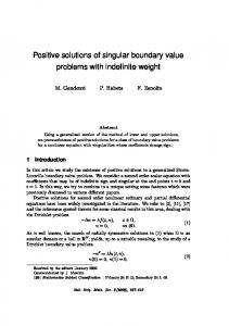
Figure 1: (a) Plot of exact, third order MADM, and second order OHAM solution of model 3.1. (b) Plot of absolute errors of OHAM and MADM with exact solutions.

2.5 0.00015

2.0 1.5

Error

y

0.00010

1.0 0.00005

0.5 0.6

0.4

0.8

1.0

0.6

0.4

x Exact MADM OHAM

0.8

1.0

x OHAM MADM

(a)

(b)

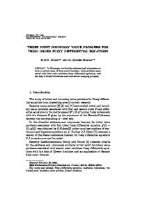
Figure 2: (a) Plot of Exact, second order MADM, second order OHAM solution of model 3.2. (b) Plot of Absolute errors of OHAM, MADM with exact solutions.


9 0.025

2.5

0.020

2.0 1.5

Error

y

1.0

0.015 0.010 0.005

0.5 0.6

0.4

0.8

1.0

0.6

0.4

x

0.8

1.0

x

Exact MADM OHAM

OHAM MADM (b)

(a)

Figure 3: (a) Plot of Exact, third order MADM, second order OHAM solution of model 3.3. (b) Plot of Absolute errors of OHAM, MADM with exact solutions.

− 0.000598031𝜉17 − 0.000244701𝜉18

− 2.66882 × 10−17 𝜉56 − 7.4357 × 10−18 𝜉57

− 0.0000869099𝜉19

+ 1.78031 × 10−18 𝜉58 − 3.07739 × 10−19 𝜉59

− 0.0000273234𝜉20 − 6.92013 × 10−6 𝜉21

+ 6.87535 × 10−20 𝜉60 + 1.26899 × 10−19 𝜉61

+ 9.73386 × 10−7 𝜉22 + 4.28328 × 10−6 𝜉23

+ 7.41807 × 10−20 𝜉62 + 2.6999 × 10−20 𝜉63

+ 4.9078 × 10−6 𝜉24 + 4.11114 × 10−6 𝜉25

+ 7.17458 × 10−21 𝜉64 + 1.49357 × 10−21 𝜉65

+ 2.87739 × 10−6 𝜉26 + 1.75577 × 10−6 𝜉27

+ 2.55087 × 10−22 𝜉66 + 3.52795 × 10−23 𝜉67

+ 9.50658 × 10−7 𝜉28 + 4.61508 × 10−7 𝜉29

− 2.35347 × 10−24 𝜉68 − 1.39052 × 10−23 𝜉69

+ 2.02183 × 10−7 𝜉30 + 7.90011 × 10−8 𝜉31

−1.48117 × 10−23 𝜉70 − 6.12864 × 10−24 𝜉71 ) 𝐾12 . (47)

+ 2.56676 × 10−8 𝜉32 + 5.3291 × 10−9 𝜉33 − 9.74128 × 10−10 𝜉34 − 2.0341 × 10−9 𝜉35 − 1.52924 × 10−9 𝜉36 − 8.57227 × 10−10 𝜉37 − 4.01512 × 10−10 𝜉38 − 1.63899 × 10−10 𝜉39 − 5.90489 × 10−11 𝜉40 − 1.79114 × 10−11 𝜉41 −12 42

− 3.55181 × 10

−13 43

𝜉 + 4.69351 × 10

𝜉

+ 1.06979 × 10−12 𝜉44 + 7.36983 × 10−13 𝜉45 + 3.68208 × 10−13 𝜉46 + 1.51155 × 10−13 𝜉47 + 5.34052 × 10−14 𝜉48 + 1.65282 × 10−14 𝜉49 −15 50

+ 4.23773 × 10

−16 51

𝜉 + 4.9859 × 10

𝜉

− 3.83336 × 10−16 𝜉52 − 3.73432 × 10−16 𝜉53 − 2.01066 × 10−16 𝜉54 − 8.11761 × 10−17 𝜉55

Solving problem (41) to (47), we obtained ̃ (𝜉) = 𝑤0 (𝜉) + 𝑤1 (𝜉, 𝐾1 ) + 𝑤2 (𝜉, 𝐾1 , 𝐾2 ) . 𝑤

(48)

We obtained the constant values of 𝐾1 and 𝐾2 as 𝐾1 = 2.7875178639324 × 10−20 , 𝐾2 = −7.889481663510912 × 10−21 .

(49)

Substituting constant values of 𝐾1 and 𝐾2 in (48) to obtain approximate solution of OHAM.

4. Conclusion Optimal homotopy asymptotic method has been applied to obtain the approximate solution of singular boundary value problems. Results have been compared with modified adomian decomposition method and with the exact solutions of proposed models. Numerical results present in Tables 1, 2, and 3 showed that this technique is fast convergent and has

10 remarkable low error than MADM. It is observed through represented plots in Figures 1(a), 2(a), and 3(a) that the presented technique is effective and reliable within bounded domain. Absolute errors plots by Figures 1(b), 2(b), and 3(b) showed the precise closeness of OHAM to exact results.

Conflict of Interests The authors declare that there is no conflict of interests regarding the publication of this paper.

References [1] Y. Q. Hasan and L. M. Zhu, “A note on the use of modified Adomian decomposition method for solving singular boundary value problems of higher-order ordinary differential equation,” Communications in Nonlinear Science and Numerical Simulation, vol. 14, no. 8, pp. 3261–3265, 2009. [2] Y. Q. Hasan and L. M. Zhu, “Solving singular boundary value problems of higher-order ordinary differential equations by modified Adomian decomposition method,” Communications in Nonlinear Science and Numerical Simulation, vol. 14, no. 6, pp. 2592–2596, 2009. [3] V. Marinca and N. Heris¸anu, “Application of optimal homotopy asymptotic method for solving nonlinear equations arising in heat transfer,” International Communications in Heat and Mass Transfer, vol. 35, no. 6, pp. 710–715, 2008. [4] V. Marinca, N. Heris¸anu, T. Dordea, and G. Madescu, “A new analytical approach to nonlinear vibration of an electrical machine,” Proceedings of the Romanian Academy A: Mathematics Physics Technical Sciences Information Science, vol. 9, no. 3, pp. 229–236, 2008. [5] V. Marinca, N. Heris¸anu, and I. Nemes¸, “Optimal homotopy asymptotic method with application to thin film flow,” Central European Journal of Physics, vol. 6, no. 3, pp. 648–653, 2008. [6] V. Marinca, N. Heris¸anu, C. Bota, and B. Marinca, “An optimal homotopy asymptotic method applied to the steady flow of a fourth-grade fluid past a porous plate,” Applied Mathematics Letters, vol. 22, no. 2, pp. 245–251, 2009. [7] M. Idrees, S. Haq, and S. Islam, “Application of optimal homotopy asymptotic method to fourth order boundary value problems,” World Applied Sciences Journal, vol. 9, no. 2, pp. 131–137, 2010. [8] M. Idrees, S. Islam, S. Haq, and S. Islam, “Application of the optimal homotopy asymptotic method to squeezing flow,” Computers & Mathematics with Applications, vol. 59, no. 12, pp. 3858– 3866, 2010. [9] M. Idrees, S. Haq, and S. Islam, “Application of optimal homotopy asymptotic method to special sixth order boundary value problems,” World Applied Sciences Journal, vol. 9, no. 2, pp. 138– 143, 2010. [10] S. Iqbal, M. Idrees, A. M. Siddiqui, and A. R. Ansari, “Some solutions of the linear and nonlinear Klein-Gordon equations using the optimal homotopy asymptotic method,” Applied Mathematics and Computation, vol. 216, no. 10, pp. 2898–2909, 2010. [11] S. Iqbal and A. Javed, “Application of optimal homotopy asymptotic method for the analytic solution of singular Lane-Emden type equation,” Applied Mathematics and Computation, vol. 217, no. 19, pp. 7753–7761, 2011.


Advances in

Operations Research Hindawi Publishing Corporation http://www.hindawi.com

Volume 2014

Advances in

Decision Sciences Hindawi Publishing Corporation http://www.hindawi.com

Volume 2014

Journal of

Applied Mathematics

Algebra

Hindawi Publishing Corporation http://www.hindawi.com


Volume 2014

Journal of

Probability and Statistics Volume 2014

The Scientific World Journal Hindawi Publishing Corporation http://www.hindawi.com


Volume 2014

International Journal of

Differential Equations Hindawi Publishing Corporation http://www.hindawi.com

Volume 2014

Volume 2014

Submit your manuscripts at http://www.hindawi.com International Journal of

Advances in

Combinatorics Hindawi Publishing Corporation http://www.hindawi.com

Mathematical Physics Hindawi Publishing Corporation http://www.hindawi.com

Volume 2014

Journal of

Complex Analysis Hindawi Publishing Corporation http://www.hindawi.com

Volume 2014

International Journal of Mathematics and Mathematical Sciences

Mathematical Problems in Engineering

Journal of

Mathematics Hindawi Publishing Corporation http://www.hindawi.com

Volume 2014


Volume 2014

Volume 2014


Volume 2014

Discrete Mathematics

Journal of

Volume 2014


Discrete Dynamics in Nature and Society

Journal of

Function Spaces Hindawi Publishing Corporation http://www.hindawi.com

Abstract and Applied Analysis

Volume 2014


Volume 2014


Volume 2014

International Journal of

Journal of

Stochastic Analysis

Optimization



Volume 2014

Volume 2014