Solving the flow fields in conduits and networks using energy minimization principle with simulated annealing Taha Sochi University College London, Department of Physics & Astronomy, Gower Street, London, WC1E 6BT Email:
[email protected].
arXiv:1408.0357v1 [physics.flu-dyn] 2 Aug 2014
Abstract In this paper, we propose and test an intuitive assumption that the pressure field in single conduits and networks of interconnected conduits adjusts itself to minimize the total energy consumption required for transporting a specific quantity of fluid. We test this assumption by using linear flow models of Newtonian fluids transported through rigid tubes and networks in conjunction with a simulated annealing (SA) protocol to minimize the total energy cost. All the results confirm our hypothesis as the SA algorithm produces very close results to those obtained from the traditional deterministic methods of identifying the flow fields by solving a set of simultaneous equations based on the conservation principles. The same results apply to electric ohmic conductors and networks of interconnected ohmic conductors. Computational experiments conducted in this regard confirm this extension. Further studies are required to test the energy minimization hypothesis for the non-linear flow systems. Keywords: fluid dynamics; pressure field; tube; network; porous media; energy minimization; simulated annealing; stochastic method; electric conductor; electric network.
1
Introduction
One of the fundamental physical principles that regulate Nature’s behavior is optimization which reflects a prejudice that leads to minimizing or maximizing selected physical quantities. For instance, Nature has a tendency to maximize the entropy of dynamic systems, as given by the second law of thermodynamics, but to minimize the passage time of light as summarized by Fermat’s least time principle. Many physical laws have been deduced or derived from optimization arguments and hence it is one of the main pillars of modern science. As a result, extensive 1
branches of mathematical and computational disciplines have been developed to deal with modeling and quantifying optimization problems with widespread applications in physical and social sciences. One of the powerful and widely used optimization methods is simulated annealing [1–3] which is a stochastic computational technique based on the physical principles of statistical mechanics. The essence of this method is to emulate the process of controlled and slow cooling of liquified substances so that they reach their minimal energy configuration in their solid state. The main advantages of simulated annealing are its simplicity and wide applicability to large classes of optimization problems as well as its high success rate of avoiding traps of local minima which other deterministic and stochastic methods are more likely to fall in. Furthermore, in many cases it is the only viable method as combinatorial enumeration and other analytical or conceptually-based methods are not viable or available in those circumstances. The main disadvantage of simulated annealing is its generally high computational cost in terms of CPU time. Although this is true for commonplace problems where alternative methods are available, in some cases simulated annealing is more efficient even in terms of CPU time when the computational cost grows exponentially and hence the cost of traditional methods, assuming their viability, becomes much higher than the cost of SA. In fact this is one of the main reasons why simulated annealing and similar stochastic methods are invented and widely used in all sorts of optimization problems as can be inferred, for instance, from the number of citations of the SA founding papers [1–3]. Regardless of this, nowadays the computational cost is a trivial factor in many cases considering the huge advances over the last few decades in the hardware and software development and the availability of multi-processor platforms, even for personal use, with relative ease of parallelization. In the present paper we suggest and examine a hypothesis that the driving field, like pressure and potential difference, in conducting elements and networks of interconnected elements will adjust itself to minimize the energy cost of transporting a given quantity of fluid through the transport device. We use simulated annealing with supporting arguments to achieve the minimization objective and establish the energy minimization hypothesis. We restrict our attention in the current investigation to the linear transport systems where the driving and induced fields are linearly correlated, such as the flow of Newtonian fluids in rigid tubes and networks of interconnected rigid tubes and the flow of electric current in ohmic components
2
and networks of interconnected ohmic components, although we will briefly discuss some issues related to the non-linear systems for the sake of completeness. The case of non-linear flow systems requires further investigation to reach definite conclusions although initial examination indicates that they are also subject to the energy minimization rules. The model that is used in the current investigation to present the energy minimization principle and elaborate the SA optimizing algorithm is from fluid mechanics, namely the aforementioned example of the flow of Newtonian fluids in rigid tubes and networks. However, since this flow model is mathematically equivalent to the flow model of electric current in ohmic devices, our investigation and conclusions will naturally extend to this case as well.
2
Method
In this study we assume a laminar, incompressible, isothermal, time-independent, pressure-driven, fully-developed flow with minor entry and exit effects. Our plan for establishing the energy minimization principle through solving the flow fields by simulated annealing is summarized in the following points 1. We establish the existence and uniqueness of the flow solution in general. 2. We explain how to adapt simulated annealing to find a flow solution in single conduits and networks of interconnected conduits. 3. We demonstrate that the solution found by simulated annealing is a correct one, it minimizes the total energy of fluid transportation, and this minimum is a global rather than a local one. As for the first point, the existence and uniqueness of flow solutions for single conduits is a thorny issue from the theoretical and mathematical viewpoint. However, it can be established by the forthcoming physical argument which we presented in the context of network discussion. Regardless of this, we can take this for granted by claiming it is an intuitive assumption. In fact most of the ongoing studies in this field should be based explicitly or implicitly on such an assumption especially the purely theoretical ones which are not supported by experimental or observational evidence. With regard to networks, the existence and uniqueness conditions can be established by the following argument assuming the existence and uniqueness of the 3
solution on their individual conduits. For the linear case, to describe such flow networks we set a system of N simultaneous linear equations in N unknowns where N is the total number of nodes in the network which includes the boundary as well as the internal nodes. The equations of the inlet and outlet nodes are derived from the boundary conditions while the equations of the internal nodes are derived from the mass conservation principle in conjunction with the characteristic flow relation that correlates the driving and induced fields, like p and Q in Hagen-Poiseuille law. Since these equations are linearly independent, due to the fact that no two equations share the same sequence of conducting elements and hence they cannot be represented as scalar multiples of each other, we have a system of N linearly independent equations in N unknowns and hence a solution does exist and it is unique according to the rules of algebra. With regard to the non-linear systems, there is no general condition that guarantees the existence or uniqueness of solution. However, physical rather than mathematical arguments can be proposed to establish the existence and uniqueness of solutions even for the non-linear systems in case such an extension is required. It can be argued that for both the linear and non-linear systems a solution should exist and it should be unique regardless of all these elaborate mathematical considerations because as long as our mathematical models reflect the essential features of the reality of these classical deterministic systems, the soundness and accuracy of these models will guarantee the existence and uniqueness conditions. Such line of reasoning should be sufficient for the purpose of establishing our energy minimization argument since we have no interest in those theoretical and mathematical subtleties. As for the second point, the time rate of energy consumption, I, of fluid transport through a conducting device considering the type of flow systems that meet our stated assumptions, is given by I = ∆p Q
(1)
where ∆p is the pressure drop across the conducting device and Q is the volumetric flow rate of the transported fluid. For a single conduit that is discretized into n sections indexed by i, the total energy consumption rate, It , is given by It =
n X i=1
4
∆pi Qi
(2)
A similar equation applies for a network of n interconnected conduits, with n standing for the number of conduits rather than sections, if only the nodal pressure values are required. If the axial pressure values at the midpoints of conduits are also required, a discretization scheme, similar to the one used for single conduits, can be used where it is needed. However, for the linear systems, only nodal pressures are necessary to compute since the midpoint values can be obtained by a simple linear interpolation scheme. The role of the simulated annealing protocol then is to find the set of pressure values, pk where k indexes the discretization and nodal points, that minimizes the rate of total energy consumption, given by Equation 2. Accordingly, the pk values can be freely adjusted by the SA routine to satisfy the minimization requirement. The exception to this is the boundary values which are held constant in all SA iterations to satisfy the imposed boundary conditions. As for the Qi values, they are computed in each SA iteration from the analytical expression of the model that correlates the volumetric flow rate to the pressure drop, i.e. Hagen-Poiseuille law in the case of Newtonian flow systems, using the most recent values of pk . Unlike the traditional solution methods, such as the residual-based Newton-Raphson technique, no conservation principle, such as mass continuity, is needed in the proposed SA solution scheme. Regarding our simulated annealing algorithm, we use a standard scheme as described by many papers and monographs written on simulated annealing and stochastic methods. Briefly, we start by initializing the pressure values, pk , randomly except the boundary ones which are set to the values required by the imposed boundary conditions. We then compute the cost function, which is initially set to a very high value, as given by Equation 2. The new pressure field solution, as defined by the set of pk values, is then accepted if the cost function obtained from the current iteration is less than the cost function of the most recently accepted solution. If the cost function of the new solution is higher, it may also be accepted but with a probability P given by P =e
It −Itm m−1 Tc
(3)
where m is an index for the current iteration and Tc is the current value of the annealing parameter (temperature) which we assume to have the same units as I. The pk values are then adjusted randomly using a random number generator and the cycle is repeated. The annealing control parameter, T , is decremented persistently as the annealing goes on. The algorithmic procedure will terminate 5
when the annealing control parameter reaches its lower limit which is normally set to virtually zero, and hence the final solution will be taken as the last accepted set of pk values according to the minimization criterion. By finding the pressure field, the volumetric flow rate field will be easily obtained from the analytical expression of the flow in single conduits that links Q to ∆p. For networks, the total inflow/outflow can be obtained by computing and summing the volumetric flow rates of the inlet/outlet boundary conduits. As well as implementing this standard SA scheme, we experimented with a number of similar SA schemes which differ in elaboration and complexity, for instance by the way that T varies or by the accepted exit condition from the interim cycles, but since they all produce very similar results we decline to include these irrelevant details. As for the third point, the verification of the single conduit solution is trivial since the axial pressure varies linearly with the conduit axial coordinate. For the networks, the obtained solution from the simulated annealing procedure can be checked for correctness by simultaneously satisfying the analytical flow relation that links Q to ∆p on each conduit plus the mass conservation principle on each internal node. Detailed explanations about these verification conditions and other related issues are given in [4]. The simulated annealing solution can also be verified more easily by comparison to the solution found by other methods, mainly the deterministic ones such as the residual-based Newton-Raphson scheme which originates from the existence and uniqueness proof that we outlined earlier. Further details about this can also be found in [4]. Since simulated annealing is essentially a minimization algorithm, the minimal energy principle is established by finding the optimal solution so no further proof is required to establish the fact that the obtained solution is not a maximum or a stationary inflection point, unlike solutions obtained by other methods where such a proof may be needed. Since this minimizing solution is the only possible solution, as established by the uniqueness condition, it should be a global rather than a local minimum since no other solution, minimizing or non-minimizing, is possible.
3
Results
The simulated annealing algorithm, which is described in the last section, was implemented in a computer code and results were obtained and analyzed using various models of fluid transport devices including rigid tubes, one-, two- and 6
three-dimensional networks of interconnected rigid tubes. The multi-dimensional networks include fractal, cubic and orthorhombic lattice models; the detailed description of these networks is given, for instance, in [4, 5]. These model tubes and networks vary in their size, geometry, connectivity, number of nodes and segments, and statistical distributions. Various boundary conditions and discretization schemes with different model Newtonian fluids were also employed in these computations. A sample of these results is given in Figures 1 and 2 and Table 1. All the results represent averaged data over many similar runs where no run has failed to meet the rigorous criteria set for accepting the solutions. As seen, the SA results agree very well with the verified deterministic solutions. One thing that should be highlighted is the general trend of increasing the size of the errors with increasing the size of the networks. The main reason is our tendency to reduce the required CPU time and hence the results can be improved if longer CPU time is allowed and more elaborate simulated annealing schemes are employed. The size of the errors in these results, nonetheless, does not affect the definite conclusion that can be drawn from this investigation about the validity of the energy minimization principle as a governing rule in determining the flow fields (p and Q) in the fluid transport systems. After all, such errors, and even larger ones, are expected to contaminate the results obtained by stochastic methods. In fact significant errors can occur even in the numerical deterministic methods although the size of the errors in the latter is usually less than that in the former. These results do not only establish the energy minimization principle but also establish a novel way for solving the flow fields in conduits and networks by stochastic methods in general and by simulated annealing in particular. Most of the reported results are obtained within seconds or minutes of CPU time on a normal laptop computer where the length of the CPU time mainly depends on the number of discretized elements in the transport device assuming the employment of the same SA parameters and scheme. Although the proposed stochastic method is generally slower than the traditional deterministic methods, it may be possible to compete with the traditional deterministic methods even in speed for very large networks especially if more elaborate SA schemes are employed. A big advantage, however, of the proposed stochastic method is the trivial memory cost; a factor based on its serial nature and the redundancy of employing a numerical solver that is usually needed in the deterministic methods. Anyway, the proposed stochastic method is a tool that is advantageous to be available to scientists and engineers and it definitely can have useful applications in some exceptional circumstances at least.
7
100 Deterministic Simulated Annealing
90 80
Axial Pressure (Pa)
70 60 50 40 30 20 10 0 0
0.02
0.04 0.06 Tube Axial Coordinate (m)
0.08
0.1
Figure 1: Comparison between the pressure field solution, as a function of the axial coordinate for a single tube, as obtained from the simulated annealing method based on the energy minimization principle and the solution obtained by interpolation or from the classical deterministic residual-based Newton-Raphson method. 1000 Deterministic Simulated Annealing
900 800
Axial Pressure (Pa)
700 600 500 400 300 200 100 0 0
0.1
0.2
0.3 0.4 0.5 0.6 Network Axial Coordinate (m)
0.7
0.8
Figure 2: Comparison between the pressure field solution, as a function of the axial coordinate for a one-dimensional network of five serially-connected tubes with different lengths and radii, as obtained from the simulated annealing method based on the energy minimization principle and the solution obtained from the classical deterministic residual-based Newton-Raphson method. 8
Table 1: Statistical distribution parameters of the percentage relative difference of the nodal pressures between the Newton-Rapson deterministic solutions and the simulated annealing solutions for a number of 2D fractal (F) and 3D orthorhombic (O) networks with the given number of segments (NS) and number of nodes (NN). The results represent averaged data over multiple runs for each network. The meaning of the statistical abbreviations are: Min for minimum, Max for maximum, SD for standard deviation, and Avr for average. Index 1 2 3 4 5 6
Type F F F F F F
NS 15 31 63 127 255 511
NN 16 32 64 128 256 512
Min -0.42 -0.70 -0.79 -0.77 -1.29 -1.87
Max 0.35 0.67 0.75 0.85 1.15 1.74
SD 0.15 0.22 0.24 0.27 0.25 0.35
Avr -0.06 -0.16 -0.05 0.19 0.07 -0.06
7 8 9 10 11 12
O O O O O O
72 99 136 176 216 275
45 60 80 96 112 140
-0.51 -0.89 -1.11 -1.42 -1.65 -1.74
0.58 0.78 1.12 1.37 1.57 1.68
0.20 0.22 0.26 0.32 0.37 0.44
0.10 -0.11 0.23 -0.17 -0.29 0.35
4
Conclusions
We demonstrated, through the use of simulated annealing, the validity of the assumption of energy minimization principle as a governing rule for the flow systems in the context of obtaining the driving and induced fields in single conduits and networks of interconnected conduits where the driving and induced fields are linearly correlated, e.g. the flow of Newtonian fluids through rigid tubes and networks or the flow of electric current through ohmic devices. All the results support the proposed energy minimization principle. There are two main outcomes of this investigation. First, a novel method for solving the flow fields that is based on a stochastic approach is proposed as an alternative to the traditional deterministic approaches such as the residual-based Newton-Raphson and finite element methods. Although this new numerical method may not be attractive in most cases where it is outperformed in speed by the traditional methods, it can surpass the other methods in other cases and may even 9
be the only viable option in some circumstances where the flow networks are very large. The second outcome, which in our view is the most important one, is the theoretical conclusion that energy minimization principle is at the heart of the flow phenomena and hence it governs the behavior of flow systems; the linear ones at least. This is inline with our previous investigations [6, 7] which are based on minimizing the total stress in the flow conduits. The current investigation may be extended in the future to the non-linear case.
Nomenclature I It P p ∆p Q T Tc
time rate of energy consumption for fluid transport time rate of total energy consumption for fluid transport probability of accepting non-minimizing SA solution pressure pressure drop across flow conduit volumetric flow rate annealing control parameter (temperature) current value of annealing control parameter
References [1] N. Metropolis; A.W. Rosenbluth; M.N. Rosenbluth; A.H. Teller; E. Teller. Equation of State Calculations by Fast Computing Machines. Journal of Chemical Physics, 21:1087–1092, 1953. [2] S. Kirkpatrick; C.D. Gelatt Jr.; M.P. Vecchi. Optimization by Simulated Annealing. Science, 220(4598):671–680, 1983. ˇ y. Thermodynamical approach to the traveling salesman problem: An [3] V. Cern´ efficient simulation algorithm. Journal of Optimization Theory and Applications, 45(1):41–51, 1985. [4] T. Sochi. Comparing Poiseuille with 1D Navier-Stokes Flow in Rigid and Distensible Tubes and Networks. Submitted, 2013. arXiv:1305.2546.
10
[5] T. Sochi. Pore-Scale Modeling of Navier-Stokes Flow in Distensible Networks and Porous Media. Computer Modeling in Engineering & Sciences (Accepted), 2014. [6] T. Sochi. Using the Euler-Lagrange variational principle to obtain flow relations for generalized Newtonian fluids. Rheologica Acta, 53(1):15–22, 2014. [7] T. Sochi. Further validation to the variational method to obtain flow relations for generalized Newtonian fluids. Submitted, 2014. arXiv:1407.1534.
11