Solving the Inverse Kinematics in Humanoid Robots: A ... - CiteSeerX

Solving the Inverse Kinematics in Humanoid Robots: A Neural Approach Javier de Lope, Telmo Zarraonandia, Rafaela Gonz´ alez-Careaga, and Dar´ıo Maravall Department of Artificial Intelligence Faculty of Computer Science Universidad Polit´ecnica de Madrid Campus de Montegancedo, 28660 Madrid, Spain {jdlope,telmoz,rafaela,dmaravall}@dia.fi.upm.es

Abstract. In this paper a method for solving the inverse kinematics of an humanoid robot based on artificial neural networks is presented. The input of the network is the desired positions and orientations of one foot with respect to the other foot. The output is the joint coordinates that make it possible to reach the goal configuration of the robot leg. To get a good set of sample data to train the neural network the direct kinematics of the robot needs to be developed, so to formulate the relationship between the joint variables and the position and orientation of the robot. Once this goal has been achieved, we need to establish the criteria we are going to use to choose from the range of possible joint configurations that fit with a particular foot position of the robot. These criteria will be used to filter all the possible configurations and retain the ones that make the robot configurations more stable in the training set.

1

Introduction

Legged robots have been one of the main topics in advanced robotic research. Projects addressing legged robots usually study the stability and mobility of these mechanisms in a range of environmental conditions for applications where wheeled robots are unsuitable. The biological inspiration of this kind of robots is also an important topic. Recent advances in mechanical and electronic robot components and the challenge of creating an anthropomorphic model of the human body have made it possible to develop humanoid robots. This work has materialized into successful projects, such as the Honda humanoids, the Waseda humanoid robots and the MIT Leg Lab robots. Lately the main interest has focused on getting the robot to remain stable as it walks in a straight line. Two methods are usually used for this purpose. The first and most widely used method aims to maintain the projection of the center of masses (COM) of the robot inside the area inscribed by the feet that are in contact with the ground. The COM represents the unique point in an object or system which can be used to describe the system’s response to external forces

2

J. de Lope et al.

and torques. The concept of COM is an average of the masses factored by the distances from a reference point. This is known as static balance. The second method, also referred to as dynamic balance, uses the zero moment point (ZMP), which is defined as the point on the ground around which the sum of all the moments of the active forces equal zero [1]. If the ZMP is within the convex hull of all contact points between the feet and the ground, the biped robot is stable and will not fall over [2, 3]. Nevertheless, linear walking is not the only type of movement the biped robot will need in order to explore the real world. It also needs to turn around, lift one foot, move sideways, step backwards, etc., and the problems involved in these movements could be quite different from those of linear walking. In this paper, we propose a method for obtaining the relative positions and orientations of a robot’s foot to achieve the above-mentioned movements. The method can be extended to other walking schemes. To achieve this kind of one-step movement, the new foot coordinates must be supplied to the control system, which will be able to determine the way the leg should move in order to place the foot in the new position and orientation. For this purpose, it will be necessary to compute the inverse kinematics of the legged robot. The proposed method for solving the inverse kinematics considers the use of an artificial neural network. This has several advantages. For example, the proposed method makes the development of an analytical solution, practically unapproachable due to the high degree of joint configurations redundancy unnecesary [4]. Furthermore, the solutions obtained are adaptive and could be implemented in hardware using the appropriate electronic device [5]. A lot of research has been done on training neural networks to resolve the inverse kinematics of a robot arm. Self-organizing maps have been widely used for encoding the sample data on a network of nodes to preserve neighborhoods. Martinetz et al. [6] propose a method to be applied to manipulators with no redundant degrees of freedom or with a redundancy resolved at training time, where a single solution along a single branch is available at run time. Jordan and Rumelhart [7] suggest first training a network to model the forward kinematics and then prepending another network to learn the identity, where the weights of the forward model are unchanged. The prepended network is able to learn the inverse. Other alternatives, like recurrent neural networks [8], are also used to learn the inverse kinematics of redundant manipulators. Kurematsu et al. [9] use a Hopfield-type neural network to solve the inverse kinematics of a simplified biped robot. The joint positions are obtained from the position of the center of gravity and the position of the toes is calculated from the equation of an inverted pendulum. The remainder of the paper is organized as follows. First, the model of the humanoid robot and the geometric space configuration are considered. Then, the stability criteria and constraints for reaching stable robot postures in the training set are examined. Next, we discuss the topology, algorithms and results

Solving the Inverse Kinematic in Humanoid Robots: A Neural Approach

3

obtained with the artificial neural nerwork. Finally, the conclusions and further work are presented.

2

Humanoid Robot Model

The model of the robot we are going to consider is based on the PINO humanoid robot [10]. The basic configuration is made up of two legs and the hip. Each leg is composed of six degrees of freedom, which are distributed as follows: two for the ankle —one rotational on the pitch axis and the other one rotational on the roll axis—, one for the knee —rotational on the pitch— and three for the hip —each of them rotational on each of the axes—. The total height of the robot is 280 mm. The links dimensions considered are 113, 65 and 102 mm for the links between the ground and the ankle, the ankle and the knee, and the knee and the hip respectively. The hip length is 200 mm [11]. A diagram of the robot legs with the dimensions of each segment is shown in Fig. 1.

Fig. 1. Model of the humanoid robot with the position and orientation of the rotational joints; the global coordinate frame considered is also represented

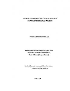
The direct kinematics of the robot as regards what the relative position and orientation of one foot from the other is can be solved easily considering our model as a robotic chain of links interconnected to one another by joints. The first link, the base coordinate frame, is the right foot of the robot. We assume it to be fixed to the ground for a given final position or movement, where the robot global coordinate frame will be placed. The last link is the left foot, which will be free to move. The assignment of the coordinate frames to the robot joints is ilustrated in Fig. 2. Obviously, to consider the positions or movements in the inverse case, that is, when the left foot is fixed to the ground and the right foot is able to move,

4

J. de Lope et al.

Fig. 2. Coordinate frames associated to the robot joints

the coordinate frames must be assigned similarly. This does not lead to any important conclusions concerning the proposed method and will not be developed at this stage of the research. The position and orientation of the left with respect to the right foot will be denoted by the homogeneous coordinate transformation matrix:  RI  RLF RI pLF RI TLF = = RI TR0 × R0 TR1 (θR1 ) × . . . × R6 TL6 (θL6 ) × 0 1 L6

TL5 (θL5 ) × . . . ×

L1

TL0 (θL0 ) ×

L0

TLF

(1)

where RI RLF denotes the rotation matrix of the left foot with respect to the right foot coordinate frame, RI pLF denotes the position matrix of the left foot with respect to the right foot coordinate frame and each i Tj denotes the homogeneous coordinate transformation matrix from link i to link j.

3

Stability Criteria and Constraints

As mentioned above, the redundancy of the degrees of freedom will mean that different joint configurations can produce the same feet position. Therefore, the criteria we will use to choose which configurations will be used as training data for the neural network need to be established. Ideally, we want the network to learn the most stable position from the range of all the possible solutions. As we are considering only the final posture of the robot, we are working with static balance: the robot would be more stable the closes the vertical projection of the COM is to the center of the support polygon formed by the feet. The height

Solving the Inverse Kinematic in Humanoid Robots: A Neural Approach

5

of the COM will also affect system stability, as the system will more stable the lower the COM. However, we are not interested in postures that place the hip too low, as we want the postures of the robot to be as natural as possible. For our simulation we are considering the distribution of the mass to be uniform for every link. We also consider that every link has a symmetrical shape. The COM of each link will then be placed at the geometric center of the link. As this applies to each robot link, we can determine the global COM of the model using: xcm

N 1 X = mi xi M i=1

ycm =

N 1 X mi yi M i=1

zcm =

N 1 X mi zi M i=1

(2)

Based on the model and direct kinematics described above, a set of angle and position pairs has been generated to be used as training data for the neural network. These positions are uniformly distributed across the coordinate range in question. The range of angle positions for each joint is shown in Table 1, and Fig. 3 shows the final positions of the free foot. Table 1. Range of angle positions for each joint θi θ1 θ2 θ3 θ4 θ5 θ6

Min −30o −30o 0 −30o 0 −45o

Max 0 30o 90o 30o 30o 0

θi θ7 θ8 θ9 θ10 θ11 θ12

Min −45o 0 −45o 0 −45o −45o

Max 0 30o 30o 90o 30o 0

At this first stage of the research, the generated postures of the robot are subject to some restrictions. The first constraint is that the two feet will always be in full contact with flat ground. The second constraint is that the knees will not be bent and the angles of the roll axis rotational joint at the hips are fixed. The artificial neural network will then learn robot postures along the roll and pitch axes, as it takes steps.

4

Artificial Neural Network

The first step is to decide which type of neural network is more suitable for this problem, then try out different parameter values like: number of neurons in each

6

J. de Lope et al.

Fig. 3. Final positions of the free foot in the training set

layer, transfer functions, size of the set of data to train the network, training algorithm to be used, and so on. After testing different kinds of artificial neural network architectures, the one we considered best suited is a two-layer backpropagation network. Properly trained backpropagation networks tend to give reasonable responses when presented with inputs that they have never seen. Characteristically, a new input will lead to an output similar to the correct output for input vectors used in training that are similar to the new input being presented. This generalization property makes it possible to train a network on a representative set of input-target pairs and get good results without training the network on all possible input-output pairs. The generated training set provides the required representative data. In fact, we have trained the network with very different sized sets of input-target pairs and the difference in the error obtained with 1000 pairs and 8000 pairs is negligible, whereas the time it takes to train the network with the bigger set of pairs increases considerably. The network architecture that is most commonly used with the backpropagation algorithm is the multilayer feedforward network. In this case, two layers are needed. Fig. 4 shows the network architecture. a1 , the output of the hidden layer, is the logsig transfer function applied to the result of the product IW1,1 (input weight matrix) by p1 (input array of 10 elements: (x, y, z) coordinates and the lengths of the 7 segments of the robot) added to b1 (biases array for the hidden layer). a2 , the output of the output layer, is the purelin transfer function applied to the result of the product LW2,1 (layer weight matrix) by a1 added to b2 (biases array for the output layer). After trying out several configurations, the hidden layer contains 35 neurons. Fewer neurons will lead to a larger number of algorithm executions to get the same error rate. If the number of neurons is over 75, the number of execution

Solving the Inverse Kinematic in Humanoid Robots: A Neural Approach

7

Fig. 4. Neural network architecture

epochs increases and execution execution increases as well. The output layer has 12 neurons, one for each angle or degree of freedom of the humanoid robot. The transfer function for the output layer has to be a purelin function, because the outputs can take any value. After trying out the purelin, tansig and logsig functions, the logsig function was chosen because it achieves a lower error rate. For the purelin function, the error goal 0.001 cannot even be reached. For the tansig and logsig functions, the error goal 0.001 is reached. After testing the network with several training algorithms appropriate for backpropagation —variable learning rate, resilient backpropagation, conjugate gradient, quasi-Newton, and Levenberg-Marquardt (LM for short)— LM was selected. LM is the fastest training algorithm for networks of moderate size. In fact, 32 epochs are needed to reach the error goal 0.001. By comparison, the epochs needed to reach an error goal of 0.01, ten times greater than the above, using the variable learning rate algorithm, is six orders of magnitude. Setting the sum-squared error goal to 0.001 and moving a training set of 1000 pairs of input-targets, the errors obtained simulating the network with a set of 75 pairs of input-targets, different from the ones used during the training stage, are as follows:

Average error Max error

Joint coordinates (degrees) 0.0193 0.3094

Obviously, errors in joint coordinates do not represent the real error in the final position of the free foot. The next table gives a summary of the average and maximum error for each axis. Note that, the average error is less than and the maximum error is close 1 millimeter.

Average error Max error

Roll (mm) Pitch (mm) Yaw (mm) 0.1005 0.1799 0.0833 0.7150 1.1030 0.6160

8

5

J. de Lope et al.

Conclusions and Further Work

A method for solving the inverse kinematics of a humanoid robot has been presented. The method is based on an artificial neural network and makes it unnecessary to develop an analytical solution for the inverse problem, which is practically unapproachable because of the redundancy in the robot joints. The proposed neural architecture for solving the inverse kinematics is able to approximate, at a low error rate, the learning samples and to generalise this knowledge to new robot postures. The error in the roll, pitch and yaw axes are close to 1 millimeter, less than the 1% considering the leg height. The next stage of our work will be to generalise the robot leg postures to maintain positions and orientations of the free foot off of the ground. These new postures will enable the robot to reach zones at different levels using both feet or even stand in stable postures on one foot. Also, the possible impact of changing the fixed foot will be considered.

References 1. Vukobratovic M., Brovac, B., Surla, D., Sotkic, D. (1990) Biped Locomotion. Springer-Verlag, Berlin 2. Huang, Q. Yokoi, K., Kajita, S., Kaneko, K., Arai, H., Koyachi, N., Tanie, K. (2001) Planning walking patterns for a biped robot. IEEE Trans. on Robotics and Automation, 17(3), 280–289 3. Furuta, T., Tawara, T., Okumura, Y., Shimizu M., Tomiyama, K. (2001) Design and construction of a series of compact humanoid robots and development of biped walk control strategies. Robotics and Autonomous Systems, 37(2–3), 81–100 4. De Lope, J., Gonz´ alez-Careaga, R., Zarraonandia, T., Maravall, D. (2003) Inverse kinematics for humanoid robots using artificial neural networks, EUROCAST 2003, Proc. of Intl. Workshop on Computer Aided Systems Theory, 216–218 5. Ossoining, H., Reisinger, E., Steger, C., Weiss, R. (1996) Design and FPGAImplementation of a Neural Network, Proc. of the 7th Int. Conf. on Signal Processing Applications & Technology, 939–943 6. Martinetz, T.M., Ritter, H.J., Schulten, K.J. (1990) Three-dimensional neural net for learning visuomotor coordination of a robot arm. IEEE Trans. on Neural Networks, 1(1), 131–136 7. Jordan, M.I., Rumelhart, D.E. (1992) Forward models: Supervised learning with a distal teacher. Cognitive Science, 16, 307–354 8. Xia, Y., Wang, J. (2001) A dual network for kinematic control of redundant robot manipulator. IEEE Trans. ond Systems, Man, and Cybernetics — Part B: Cybernetics, 31(1), 147–154 9. Kurematsu, Y., Maeda, T., Kitamura, S. (1993) Autonomous trajectory generation of a biped locomotive robot. IEEE Int. Conf. on Neural Networks, 1961–1966 10. Yamasaki, F., Miyashita, T., Matsui, T., Kitano, H. (2000) PINO, The humanoid that walk, Proc. of The First IEEE-RAS Int. Conf. on Humanoid Robots, MIT 11. Endo, K., Maeno, T., Kitano, H. (2002) Co-evolution of Morphology and Walking Pattern of Biped Humanoid Robot using Evolutionary Computation — Consideration of characteristic of the servomotors—, IEEE/RSJ Int. Conf. on Intelligent Robots and Systems, 2678–2683