The problems solved concern Wien's displacement law and the fringing fields of a capacitor, the latter problem being representative of some problems solved ...
1
Some Applications of the Lambert Function to Physics
W
S. R. Valluri, D. J. Jeffrey, R. M. Corless
Abstract: Two standard physics problems are solved in terms of the Lambert W function, in order to show the applicability of this recently defined function to physics. Other applications of the function are cited, but not described. The problems solved concern Wien’s displacement law and the fringing fields of a capacitor, the latter problem being representative of some problems solved using conformal transformations. The physical content of the solutions remains unchanged, but they gain a new elegance and convenience.
1. Introduction Many physicists have experienced, during their education, the surprise of seeing a known mathematical function appear in a new physical context. An example in elementary physics is one that arises when students are first taught about simple harmonic motion. We hope that some readers can remember their amazement on learning that the motion of objects bobbing on springs, or moving in circles, can be described using trigonometric functions. At the time, they might have wondered, “The functions sine and cosine are used for all of those triangle problems in geometry class; there are no triangles here”. A recent example of the same phenomenon is the discovery that a function called the Lambert W function has applications in a number of areas of physics, even though it was first defined by a computer scientist for the purpose of counting search trees. Several well-known problems in electrostatics and in quantum mechanics can be solved with greater facility using it. In addition to presenting these problems, we give references to other, less elementary, applications. Mathematical functions do not by themselves uncover new physics — rather they assist the physicist by facilitating numerical and algebraic computations. A physicist therefore demands several things of any new function before taking the time to learn about it. The first feature it should have is that it is likely to have some general applicability. Abramowitz & Stegun [1] is full of functions that most of us would prefer not to know anything about; we only want to know about functions that will probably prove useful. Each person will draw the line between useful and not useful at a different place. The second feature is that there should be convenient access to numerical evaluation and to pertinent algebraic properties. A function that cannot be worked with easily is not much use. Many readers will be familiar with the conference scene in which a colleague asks you whether you know of a computer program to calculate values of the Chepooka function1. You probably reply that you yourself need a reference on the asymptotic properties of the Horrorshow function, at which point the two of you change the topic of conversation. Until the advent of the scientific calculator, even trigonometric functions and logarithms were not so easy to evaluate. The Lambert W function is a function that meets the criteria just listed. It first received a name in 1
The names of these fictitious functions are inspired by the novel A Clockwork Orange.
Valluri, Jeffrey and Corless. The University of Western Ontario, London, Canada N6A 5B7 valluri,djeffrey,r orless �julian.uwo. a
f
Can. J. Phys. : 1–8 ()
g
NRC Canada
2
Can. J. Phys. Vol. ,
the early 1980s, when the program Maple defined a function that was named simply W . An historical search, conducted while writing an account of this function [4], found work by the eighteenth century scientist J. H. Lambert that foreshadowed the definition of the function; even though his work did not actually define the function, W was named in his honour. The same search uncovered a fortuitous reason for calling the function W , in that E. M. Wright, a mathematician known for his book with Hardy on pure mathematics, studied the complex values of the function, again without naming it. The function is not connected with the Lambert transform of a function, which has been defined independently [13]. The definition of W is that it is the function that solves the equation W eW
=z;
(1)
where z is a complex number. This equation always has an infinite number of solutions, most of them complex, and so W is a multivalued function. The different possible solutions are labelled by an integer variable called the branch of W . Thus the proper way to talk about the solutions of (1) is to say that they are Wk (z ), for any k = 0; �1; �2; etc. There is always special interest in solutions that are purely real, and so we note immediately that when z is a real number, equation (1) can have either two real solutions, in which case they are W0 (z ) and W 1 (z ), or it can have only one real solution, this being W0 (z ) [with W 1 (z ) now being complex], or no real solution. Even if z is real, the branches other than k = 0; 1 are always complex. Admittedly, W does not yet appear on any pocket calculator, but it is known to the computing systems Maple, Macsyma and Mathematica (in the case of Mathematica, the function is called Produ tLog). Therefore, as soon as a problem is solved in terms of W , numerical values, plots, derivatives and integrals can be easily obtained. The first physics problem to be solved explicitly in terms of W was one in which the exchange forces between two nuclei within the hydrogen molecular ion (H2+ ) were calculated [11]; this, however, is a long and difficult calculation (and it has already been published) so instead of describing it, we have taken two much simpler problems from standard physics textbooks, problems that many students meet in their physics education, and we have expressed the solutions in terms of W . As mentioned above, the physical content does not change, only the ease of working. An additional point of interest is the fact that the electrostatic application helps to justify a mathematical decision concerning the definition of W that was originally taken entirely on aesthetic (in a mathematical sense) grounds.
2. Wien’s displacement law The spectral distribution of black body radiation is a function of the wavelength � and absolute temperature T , and is described by �(�; T ), defined such that �(�; T ) d� is the power emitted in a wavelength interval d� per unit area from a black body at absolute temperature T . The wavelength �max at which � is a maximum obeys Wien’s displacement law �max T = b, where b is Wien’s displacement constant [3]. This law was proposed by Wien in 1893 from general thermodynamic arguments. Once Planck’s spectral distribution law is known, Wien’s law can be deduced and the value of b determined. The Planck Spectral distribution law is
(
� �; T
�h =�5 ) = exp(8h =�kT ) 1:
The value of � for which this function is a maximum can be obtained by solving ��=�� simplification, this leads to the equation
5 exp
�
h �kT
�
+ 5 + exp
�
h �kT
�
h �kT
= 0. After
=0:
which, on the substitution x = h =�kT , can be written concisely as the transcendental equation
(x 5)ex = 5 :
(2) NRC Canada
Valluri, Jeffrey, Corless
3
This equation has the trivial solution x = 0 and the nontrivial one x
= 5 + W0 ( 5e 5) :
Therefore Wien’s law is obtained with a new expression for Wien’s displacement constant: b
= 2:893 � 10 3 mK: = 5 + Wh =k 5) 0 ( 5e
(3)
In the past, one would have obtained the numerical value of the law by programming a NewtonRaphson or similar solver on equation (2); now one can start up a computer package and obtain the value without programming. Time is saved not only because no programming is needed, but also because the system developers have implemented the fastest and most accurate method of evaluation.
3. Capacitor fields and conformal mapping The equipotential lines that are to be calculated are shown in figure 1 in the top set of axes. We see there the fringing field at the edge of a two-dimensional parallel-plate capacitor. The plates are assumed to be semi-infinite, and at potentials �V . The coordinates of any point in the plane are expressed as a complex number: � = � + i� . The plane is therefore called the � -plane, and what is required is a function �(� ) giving the electric potential at any point. This function is usually obtained using conformal-mapping techniques [12]. In general, conformal techniques solve a problem by relating its geometry to a simpler geometry in which the governing equations are easily solved. In the present case, the simpler geometry is shown at the bottom of figure 1 and consists of two parallel infinite planes. What we are given is a transformation � = f (z ) and a solution �(z ), valid in the z -plane. To stay with generalities for a moment, before giving the specific details of this problem, we notice that the transformation has been written � = f (z ). This means that the solution is obtained as a pair of equations:
�(� ) = � =
() f (z ) :
� z ;
In order to obtain the desired �(� ) explicitly, one must invert the transformation f to eliminate z . This is usually not easy to do. We now give the details of the problem at hand. The conformal transformation that is used is [12] �
= 1 + z + ez :
(4)
This is a member of the Schwarz-Christoffel family of transformations [8]; also � (z ) obeys a differential equation of Bernoulli type. The z -plane is shown in figure 1, filled with horizontal lines. Each line has the (complex) equation z = x + iK , where x varies and K is the constant describing the line. The plates are given by K = �� . The effect of the transformation is to map the straight lines in the bottom set of axes to the curves in the top set of axes. If z = x + iy , the potential in the z -plane is � = V y=� = V =z=� , where =z means imaginary part of z . Therefore, given a point z between the infinite plates, we can find the corresponding � coordinate and then know the potential there. As foreshadowed, the unsatisfactory part of the solution is the fact that we do not get the solution as a function of � . Given a point � , we must solve (4) to find z . In general, conformal transformations do not have simple inverses, and the computations must be programmed as a root-finding exercise. In the past, the problem at hand was one more example of this, but now the definition and implementation of Lambert W have made it possible to invert (4) explicitly. During the solution, an arbitrary integer k is introduced to indicate the existence of multiple solutions. We proceed: �
1 =
z
+ ez ; NRC Canada
4
Can. J. Phys. Vol. ,
4
2
Physical plane: –2
0
–1
1
2
(The � -plane) –2
�
=)
–4
= 1 + z + ez
3
2
1
Starting solution: –3
–2
–1
0
1
2
3
(The z -plane) –1
–2
–3
Fig. 1. The top set of axes (the � -plane) show the edge of a parallel-plate capacitor. The plates are the heavy lines. The equipotential lines of the fringing field are shown and are calculated as images of horizontal grid lines in the z -plane. The bottom set of axes show the z -plane, which is mapped to the � -plane by � = 1 + z + ez .
NRC Canada
Valluri, Jeffrey, Corless e�
1
�
1
ez z z
5
z
= = = =
e z ee ;
( 1) ; Wk (e� 1 ) ; � 1 Wk (e� 1 ) : Wk e�
(5)
Some further analysis (not given here) shows that the restriction � < =z < � implies that the branch index k is also specified, once � is known; moreover, we can give an analytic formula for this, in terms of K, the unwinding number [5, 7]. The expression is �
k
= K (� ) = =�2� �
�
:
(6)
Here the symbol d e denotes the ceiling function, which is the integer obtained by rounding up (as opposed to floor which is obtained by rounding down). Figure 2 shows how the inverse transformation works. Recalling the notation, � = � + i� , we divide the � -plane into strips of width 2� . The main strip between the plates, and extending to the right, is � < � < � and is shown containing solid lines. The strips 3� < � < � and � < � < 3� are shown containing dashed lines. Each strip is transformed using a different branch of W , the one with index k = K(� ), onto a distinct portion of the strip � < =z < � . The portions of the strip thus mapped are symmetric, in the sense that W k and Wk map into regions symmetric about the real z axis. In summary, we have derived the following new analytical formula for the solution for the fringing fields of a semi-infinite capacitor. The potential at the point � is
� = (V =�)=
�
�
1
WK(� ) e�
1
��
:
(7)
As stated in the introduction, for this formula to be actually useful, it must be easily evaluated. Although the number of computer packages that contain W built-in is still small, the packages are among the most popular ones at the moment. Therefore this formula is genuinely computational. This application to conformal mappings adds an interesting postscript to the history of the definition of W . The equation (1) does not by itself completely define the branches of W [4, 6], as explained in the next section. The definition finally chosen in [4] and implemented in the various mathematical packages was chosen purely to obtain simple asymptotic expansions for W (z ) for large z . The present physics application confirms the utility of the choice made, because any other choice would force a more complicated expression to be used in place of (7). Once again, as in the past, physics and mathematics agree on the best definitions.
4. Further properties of
W
Rather than continue with more descriptions of problems (more references are given below), we assume in this section that the case for knowing something about W has been made, and amplify the introductory description of its properties. An obvious starting point is a graph of its real values. The two real branches are shown in Figure 3, the principal branch W0 (x) is the solid line, and the branch W 1 (x) is the dashed line. Some numerical values are also given in table 1. Most readers will not be surprised that W can be differentiated: W 0 = e W =(1 + W ), but may be surprised that functions containing it can be integrated. Z
()
W x dx
Z
()
xW x dx
= (W 2 (x) W (x) + 1)eW (x) + C = 18 (2W (x) 1)(2W 2 (x) + 1)e2W (x) + C :
(8) (9) NRC Canada
6
Can. J. Phys. Vol. ,
These lines transformed using W1
6
4
Physical plane: Lines in � -plane
2
These lines transformed –3
–2
–1
where values of potential are required
0
1
2
3
using W0
–2
–4
These lines transformed
=� 1
(
W e�
(=
z
1
using W
–6
1
)
3
2
1
Lines where evaluations are made in z -plane
–3
–2
–1
0
1
2
3
–1
–2
–3
Fig. 2. The top and bottom sets of axes again show the � - and z -planes. Now the transformation proceeds from top to bottom using the inverse mapping z = � 1 WK(� ) (e� 1 ).
NRC Canada
Valluri, Jeffrey, Corless
7
W 1 −1/e
x
−1
1
2
3
−1 −2 −3 −4
Fig. 3. The real values of the Lambert W function. The solid line shows W0 and the dashed line W
1.
Many other algebraic properties have been found [4], but we quote only one more that might be useful in physical applications: an asymptotic formula for large (complex) z .
( ) � ln z + 2�ik ln(ln z + 2�ik) ; (10) where ln z is the principal branch of the (complex) natural logarithm (i.e., the function implemented in Wk z
software packages that support complex functions). Any physicist using W also benefits from lengthy studies of the quickest way to evaluate the function accurately. The basic strategy is to use the asymptotic formula to obtain a starting estimate for an iterative scheme similar to Newton iteration. Most physicists would jump to a Newton scheme if asked to evaluate the function without help, but the packages have optimized this strategy to ensure accuracy (always getting the branch correct, for example) and speed. The liberty in assigning the branches of W that was referred to above can be illustrated using the values of W given in table 1. The reader can notice that although 14 +i and 14 i are complex conjugates, it is not the case that W1 ( 14 + i) and W1 ( 14 i) are correspondingly complex conjugates. The branches of W could be assigned so that this relation became true, and indeed, an early version of Maple did assign branches that way. Such a definition, however, would not satisfy the simple asymptotic relation (10). Our physics application has confirmed that the symmetries as displayed in the table are the best ones to have.
5. Concluding remarks We have discussed two standard problems of physics in which the Lambert W function can be used. They are not the only two problems in which W arises. For example, Adler and Piran [2] used W in their work on effective action models for a system of heavy antiquark and light scalar quark; they were working about the time when the function was named and before its properties had been set out, and so they did not benefit from the convenience they would now have. In their model, as well as in nonlinear quantum electrodynamics, the nonlinear dielectric constant has a logarithmic dependence on the applied electric field, which meant that W could be used to describe the electric displacement. Mann and Ohta [9, 10] have used W to elucidate the physics involved in their study of Lagrangians for two-dimensional gravity. NRC Canada
8
Can. J. Phys. Vol. , x e
W0 (x)
1
0:5671
0
0
W
1 (x)
0:5321
1
4:597 i
1:534
4:375 i
complex infinity
W1 (x) 0:5321 + 4:597 i 1:534 + 4:375 i
complex infinity
1=e
1
1
3:089 + 7:462 i
1=4
0:3574
2:153
3:490 + 7:414 i
1=4 + i 1=4 i
0:3169 + 0:6807 i 0:3169
0:6807 i
0:9667 1:843
2:532 i 6:241 i
1:843 + 6:241 i 0:9667 + 2:532 i
Table 1. Some exact and approximate values for the Lambert W function. Of the infinite number of branches Wk , we tabulate 3 branches. The entries ‘complex infinity’ mean that the values of W 1 (0) and W1 (0) have infinite real part, but their imaginary parts depend upon the direction in which 0 is approached.
The Lambert W function has a rich variety of applications ranging from physics and computer science, to statistics and biology. Examples include the calculations of partitions in number theory, water-wave heights in oceanography, enumeration of trees in combinatorics and distribution of cycles in random mappings, the thrust specific consumption in aeronautics, enzyme kinetics, exchange forces between two nuclei within the hydrogen molecular ion H2+ , movement of water in soil, detailed study of Newton’s apsidal precession theorem, relativistic theories of gravity, and statistical distributions. There is a variety of other problems where this function is applicable and where it clarifies aspects of the physics. Many more such uses are being identified in physics and also other fields of endeavour.
6. Acknowledgements We would like to thank Khoa Nguyen (Applied Mathematics, UWO) for leading us to the reference of Adler and Piran. We would also like to thank Professor W. E. Baylis (Physics, Univ. Windsor) for several useful suggestions to improve the manuscript. Ram Valluri would like to thank Professors Paul Sullivan (Chair, Applied Mathematics, UWO), Mike Cottam (Chair, Physics and Astronomy, UWO) and Roland Haines (Associate Dean of Science, UWO) for their support and encouragement.
References 1. A BRAMOWITZ , M., AND S TEGUN , I. J. Handbook of Mathematical Functions. Dover, 1965. 2. A DLER , S. L., AND P IRAN , T. Relaxation methods for gauge field equilibrium equations. Reviews of Modern Physics 56 (1984), 1–40. 3. B RANSDEN , B., AND J OACHAIN , C. Introduction to Quantum Mechanics. Longman, Harlow, U.K., 1989. 4. C ORLESS , R. M., G ONNET, G. H., H ARE , D. E., J EFFREY, D. J., AND K NUTH , D. E. On the Lambert W function. Advances Computational Maths 5 (1996), 329–359. 5. C ORLESS , R. M., AND J EFFREY, D. J. The unwinding number. S IGSAM Bulletin 30, 2 (June 1996), 28–35. 2 6. G OSPER J R ., R. W. The solutions of yey = x and yey = x. S IGSAM Bulletin 32, 1 (Mar 1998), 8–10. 7. J EFFREY, D. J., H ARE , D. E. G., AND C ORLESS , R. M. “Unwinding the branches of the Lambert W function”. Mathematical Scientist 21 (1996), 1–7. 8. KOBER , H. Dictionary of conformal representations. Dover, New York, 1957. 9. M ANN , R. B., AND O HTA , T. Classical and Quantum Gravity 14 (1997), 1259–1263. 10. M ANN , R. B., AND O HTA , T. Physical Review D 55 (1997), 4723. 11. S COTT, T. C., BABB , J. F., DALGARNO , A., AND M ORGAN III, J. D. Resolution of a paradox in the calculation of exchange forces for h+ 2 . Chemical Physics Letters 203 (1993), 175–183. 12. VANDERLINDE , J. Classical Electromagnetic Theory. John Wiley and Sons, Inc, Toronto, Canada, 1993. 13. Z AYED , A. I. Handbook of function and generalized function transformations. CRC Press, Boca Raton, Florida, 1996. NRC Canada