We first define Markovian discrete branching processes in discrete time, known
as ... Last, we introduce the coalescent point process of branching trees : on a ...
Some aspects of discrete branching processes ∗ Amaury Lambert† April 2010
Abstract We first define Markovian discrete branching processes in discrete time, known as Bienaym´e-Galton-Watson (BGW) processes. We review some basic results like the extinctionexpansion dichotomy, computation of the one-dimensional marginals using generating functions, as well as of the extinction probability. We introduce the BGW process with immigration and state three limit theorems. We define the notion of quasi-stationarity for Markov chains and provide the basic results in the case of a finite-state space. In the case of BGW processes, we characterize Yaglom quasi-stationary limit (one-dimensional distribution conditional on non extinction) and the Q-process (process conditioned on non-extinction in the distant future). Then we show how to code the genealogy of a BGW tree thanks to a killed random walk. The law of the total progeny of the tree is studied thanks to this correspondence. Alternative proofs are given via Dwass–Kemperman identity and the ballot theorem. Last, we introduce the coalescent point process of branching trees : on a representation of the quasi-stationary genealogy of an infinite population, which is also doubly infinite in time; on splitting trees, which are those trees whose width process is a (generally not Markovian) binary, homogeneous Crump–Mode–Jagers process. For the interested reader, the following books are classical references on branching models and random trees : [4, 5, 8, 11, 15, 16, 21].
Contents 1 The Bienaym´ e–Galton–Watson model 1.1 Definitions . . . . . . . . . . . . . . . . 1.2 Some computations . . . . . . . . . . . 1.2.1 Exercises . . . . . . . . . . . . 1.2.2 Examples . . . . . . . . . . . . 1.3 BGW process with immigration . . . . 1.4 Kesten–Stigum theorem . . . . . . . .
. . . . . .
. . . . . .
. . . . . .
. . . . . .
. . . . . .
. . . . . .
. . . . . .
. . . . . .
. . . . . .
. . . . . .
. . . . . .
. . . . . .
. . . . . .
. . . . . .
. . . . . .
. . . . . .
. . . . . .
. . . . . .
. . . . . .
. . . . . .
. . . . . .
. . . . . .
. . . . . .
2 2 5 5 5 5 6
∗ This document will serve as a support for 4 lectures given at the CIMPA school in April 2010 in Saint–Louis, Senegal. Sections 1 and 2 contain previously published material [28]. † Universit´e Paris 6 Pierre et Marie Curie, France.
1
2 Quasi–stationarity 2.1 Quasi-stationarity in Markov chains . . 2.2 Finite state-space and Perron–Frobenius 2.3 Quasi-stationarity in BGW processes . . 2.3.1 Yaglom limit . . . . . . . . . . . 2.3.2 The Q-process . . . . . . . . . .
. . . . theory . . . . . . . . . . . .
. . . . .
. . . . .
. . . . .
. . . . .
. . . . .
. . . . .
. . . . .
. . . . .
. . . . .
. . . . .
. . . . .
. . . . .
. . . . .
. . . . .
. . . . .
. . . . .
. . . . .
. . . . .
7 7 7 8 8 10
3 Random walks and BGW trees 3.1 The Lukasiewicz path . . . . . . . 3.2 Kemperman’s formula . . . . . . . 3.2.1 Cyclic shifts . . . . . . . . . 3.2.2 Lagrange inversion formula 3.2.3 Dwass proof . . . . . . . . .
. . . . .
. . . . .
. . . . .
. . . . .
. . . . .
. . . . .
. . . . .
. . . . .
. . . . .
. . . . .
. . . . .
. . . . .
. . . . .
. . . . .
. . . . .
. . . . .
. . . . .
. . . . .
. . . . .
11 11 13 13 15 15
4 Coalescent point processes 4.1 The coalescent point process of quasi-stationary BGW trees 4.1.1 A doubly infinite population . . . . . . . . . . . . . 4.1.2 The coalescent point process . . . . . . . . . . . . . 4.1.3 Disintegration of the quasi-stationary distribution . 4.2 Splitting trees . . . . . . . . . . . . . . . . . . . . . . . . . .
. . . . .
. . . . .
. . . . .
. . . . .
. . . . .
. . . . .
. . . . .
. . . . .
. . . . .
. . . . .
. . . . .
17 17 17 18 19 20
1
. . . . .
. . . . .
. . . . .
. . . . .
. . . . .
. . . . .
The Bienaym´ e–Galton–Watson model
Historically, the Bienaym´e–Galton–Watson model was the first stochastic model of population dynamics [20, 43].
1.1
Definitions
Assume we are given the law of a random integer ξ pk := P(ξ = k)
k ≥ 0,
where p0 and p1 will always be assumed to be both different from 0 and 1. The population size at time n will be denoted by Zn . Assume that at each time n, individuals in the population are randomly labelled i = 1, . . . , Zn . The dynamics of the BGW tree are given by the following rules (see Fig. 1). • generation n + 1 is made up of the offspring of individuals from generation n • conditional on Zn , for any 1 ≤ i ≤ Zn , individual i from generation n begets a number ξi of offspring • the ξi ’s are independent and all distributed as ξ. The Markov chain (Zn ; n ≥ 0) is called the BGW process. It contains less information than the whole BGW tree, which provides the whole genealogical information. If Z(x) denotes a BGW
2
process started with Z0 = x individuals, then it is straightforward to check that the following branching property holds L ˜ Z(x + y) = Z(x) + Z(y), (1) where Z˜ is an independent copy of Z. In general, stochastic processes that satisfy (1) are called branching processes.
✲
0
1
2
3
4
5
6
Figure 1: A Bienaym´e–Galton–Watson tree through 6 generations, starting from one ancestor (crosses mean death with zero offspring; vertical axis has no meaning). It is convenient to consider the generating function f of ξ (see Fig. 2) � f (s) := E(sξ ) = pk s k s ∈ [0, 1], k≥0
as well as its expectation m := E(ξ) = f � (1−) ∈ (0, +∞].
We write Pz for the conditional probability measure P(· | Z0 = z). Unless otherwise specified, P will stand for P1 . Proposition 1.1 The generating function of Zn is given by Ez (sZn ) = fn (s)z
s ∈ [0, 1],
where fn is the n-th iterate of f with itself. In particular, E(Zn | Z0 = z) = mn z.
3
(2)
f (s) 1 ✻ m1
q
✲ s
�
1
0
�
� �
�
� �
� �
�
� � �
✲ s
q
(a)
1
(b)
Figure 2: Graph of the probability generating function f (a) for a subcritical BGW tree (b) for a supercritical BGW tree, with extinction probability q shown. Proof.
One can compute the generating function of Zn+1 conditional on Zn = z as E(sZn+1 | Zn = z) = E(s
�z
i=1 ξi
)=
z �
E(sξi ) = f (s)z .
i=1
Iterating the last displayed equation then yields (2). Differentiating (2) w.r.t. s and letting s tend to 1, gives the formula for the expectation. ✷ We say that extinction occurs if Z hits 0, and denote {Ext} this event. Before stating the next result, recall that f is an increasing, convex function such that f (1) = 1. As a consequence, f has at most 2 fixed points in [0, 1]. More specifically, 1 is the only fixed point of f in [0,1] if m ≤ 1, and if m > 1, f has another distinct fixed point traditionally denoted by q (see Fig. 2). Definition 1.2 A BGW tree is said subcritical if m < 1, critical if m = 1, and supercritical if m > 1. Theorem 1.3 We have Pz (Ext) = q z , which equals 1 in the subcritical and critical cases. In the supercritical case, limn→∞ Zn = +∞ conditionally on non-extinction a.s. Proof. Notice that Z is an irreducible Markov chain with two classes. Since {0} is an accessible, absorbing state, the class {1, 2, 3, . . .} is transient, and the first part of the theorem is proved. To get the second part, observe that {Ext} is the increasing union, as n ↑ ∞, of the events {Zn = 0}, so that P(Ext) = lim ↑ P(Zn = 0). n→∞
4
Thanks to (2), Pz (Zn = 0) = fn (0)z , so that P(Ext) is the limit of the sequence (qn )n defined recursively as q0 = 0 and qn+1 = f (qn ). By continuity of f , this limit is a fixed point of f , so it belongs to {q, 1}. But 0 = q0 < q so taking images by the increasing function f and iterating, one gets the double inequality qn < q ≤ 1, which ends the proof. ✷
1.2 1.2.1
Some computations Exercises
Exercise 1 Assuming that σ 2 := Var(ξ) is finite, prove that � 2 n−1 mn −1 σ m if m−1 Var(Zn | Z0 = 1) = 2 nσ if
m �= 1 m = 1.
Exercise 2 Assume m > 1. Show that conditional on {Ext}, Z has the same law as the subcritical branching process Z � with offspring distribution p�k = q k−1 pk , whose generating function is f � (s) = q −1 f (qs) s ∈ [0, 1]. This subcritical branching process is called the dual process. Exercise 3 State and prove a similar result for the subtree of infinite lines of descent conditional on {Extc }. 1.2.2
Examples
Binary. Assume pk = 0 for all k ≥ 3, and call this model Binary(p0 , p1 , p2 ). The process is supercritical iff p2 > p0 , and in that case, the extinction probability is q = p0 /p2 . The dual process is Binary(p2 , p1 , p0 ). Geometric. Assume pk = (1 − a)ak , and call this model Geometric(a). We have m = a/(1 − a). The process is supercritical iff a > 1/2, and in that case, the extinction probability is q = (1 − a)/a. The dual process is Geometric(1 − a). Poisson. Assume pk = e−a ak /k!, and call this model P oisson(a). The process is supercritical iff a > 1, and in that case, we have the inequality q < 1/a. The dual process is P oisson(qa). Linear fractional. Assume p0 = b and pk = (1 − b)(1 − a)ak−1 for k ≥ 1. Call this model LF (a, b). We have m = (1 − b)/(1 − a). The process is supercritical iff a > b, and in that case, the extinction probability is q = b/a. The dual process is LF (b, a). This example has very interesting features, see e.g. section I.4 of [4].
1.3
BGW process with immigration
Assume that in addition to the law of a random integer ξ (offspring distribution) with generating function f , we are also given the law of a random integer ζ (immigration law) with generating function g. The dynamics of the BGW tree with immigration is given by the following rules
5
• generation n + 1 is made up of the offspring of individuals from generation n and of a random number ζn+1 of immigrants, where the ζi ’s are independent and all distributed as ζ • conditional on Zn , for any 1 ≤ i ≤ Zn , individual i from generation n begets a number ξi of offspring • the ξi ’s are independent and all distributed as ξ. It is important to understand that to each immigrant is given an independent BGW descendant tree with the same offspring distribution. The population size process (Zn ; n ≥ 0) of this model is a discrete-time Markov chain called BGW process with immigration. It is straightforward that Ez (sZ1 ) = g(s)f (s)z . Iterating this last equation yields Ez (sZn ) = fn (s)z
n−1 � k=0
g ◦ fk (s)
s ∈ [0, 1].
(3)
The following theorem concerns the asymptotic growth of subcritical BGW processes with immigration. Theorem 1.4 (Heathcote [17]) Assume m < 1. Then the following dichotomy holds E(log+ ζ) < ∞ ⇒ (Zn ) converges in distribution E(log+ ζ) = ∞ ⇒ (Zn ) converges in probability to + ∞. Theorem 1.5 (Seneta [39]) Assume m > 1. Then the following dichotomy holds E(log+ ζ) < ∞ ⇒ limn→∞ m−n Zn exists and is finite a.s. E(log+ ζ) = ∞ ⇒ lim supn→∞ c−n Zn = ∞ for any positive c a.s. For recent proofs of these theorems, see [34], where they are inspired from [2]. For yet another formulation, see [28].
1.4
Kesten–Stigum theorem
Assume that 1 < m < ∞ and set Wn := m−n Zn . It is elementary to check that (Wn ; n ≥ 0) is a nonnegative martingale, so it converges a.s. to a nonnegative random variable W W := lim
n→∞
Zn . mn
To be sure that the geometric growth at rate m is the correct asymptotic growth for the BGW process, one has to make sure that W = 0 (if and) only if extinction occurs. Theorem 1.6 (Kesten–Stigum [25]) Either P(W = 0) = q or P(W = 0) = 1. The following are equivalent (i) P(W = 0) = q (ii) E(W ) = 1 (iii) (Wn ) converges in L1 (iv) E(ξ log+ ξ) < ∞. 6
For a recent generalization of this theorem to more dimensions, see [3]. For a recent proof, see [33]. Results for (sub)critical processes on the asymptotic decay of P(Zn �= 0), as n → ∞, will be displayed in the following section. Exercise 4 Prove that (Wn ; n ≥ 0) indeed is a martingale and that P(W = 0) is a fixed point of f . Under the assumption E(ξ 2 ) < ∞, show that (Wn ) is bounded in L2 , and deduce (iii), (ii) and (i) (this was done by Kolmogorov in 1938 [27]).
2 2.1
Quasi–stationarity Quasi-stationarity in Markov chains
Let X be a Markov chain on the non-negative integers for which 0 is one (and the only) accessible absorbing state. Then the only stationary probability of X is the Dirac mass at 0. A quasi-stationary distribution (QSD) is a probability measure ν satisfying Pν (Xn ∈ A | Xn �= 0) = ν(A)
n ≥ 0.
(4)
Hereafter, we will only consider quasi-stationary probabilities. A quasi-stationary distribution may not be unique, but a specific candidate is defined (if it exists) as the law of Υ, where P(Υ ∈ A) := lim Px (Xn ∈ A | Xn �= 0), t→∞
for some Dirac initial condition x �= 0. The r.v. Υ is sometimes called the Yaglom limit, in reference to the proof of this result for BGW processes, attributed to A.M. Yaglom [44]. Then by application of the simple Markov property, Pν (T ≥ n + k) = Pν (T ≥ n)Pν (T ≥ k), so that the extinction time T under Pν has a geometric distribution. Further set P↑x (Θ) := lim Px (Θ | Xn+k �= 0), k→∞
defined, if it exists, for any Θ ∈ Fn . Thus resulting law P↑ is that of a (possibly dishonest) Markov process X ↑ , called the Q-process.
2.2
Finite state-space and Perron–Frobenius theory
A comprehensive account on the applications of Perron–Frobenius theory to Markov chains is the book by E. Seneta [40]. Let X be a Markov chain on {0, 1, . . . , N } that has two communication classes, namely {0} and {1, . . . , N }. We assume further that 0 is accessible from the other class. Next, let P be the transition matrix, that is, the matrix with generic element pij := Pi (X1 = j) (row i and column j), and let Q be the square matrix of order N obtained from P by deleting its first row and its first column. In particular, Pi (Xn = j) = qij (n)
i, j ≥ 1,
where qij (n) is the generic element of the matrix Qn (row i and column j). 7
Recall that the eigenvalue with maximal modulus of a matrix with nonnegative entries is real and nonnegative, and is called the dominant eigenvalue. The dominant eigenvalue of P is 1, but that of Q is strictly less than 1. Now because we have assumed that all nonzero states communicate, Q is regular, so thanks to the Perron–Frobenius theorem, its dominant eigenvalue, say λ ∈ (0, 1) has multiplicity 1. We write v for its right eigenvector (column vector with positive entries) and u for its left eigenvector (row vector with positive entries), normalized so that � � ui = 1 and ui vi = 1. i≥1
i≥1
Theorem 2.1 Let (Xn ; n ≥ 0) be a Markov chain in {0, 1, . . . , N } absorbed at 0, such that 0 is accessible and all nonzero states communicate. Then X has a Yaglom limit Υ given by P(Υ = j) = uj
j ≥ 1,
and there is a Q-process X ↑ whose transition probabilities are given by Pi (Xn↑ = j) =
vj −n λ Pi (Xn = j) vi
i, j ≥ 1.
↑ In addition, the Q-process converges in distribution to the r.v. X∞ with law ↑ P(X∞ = j) = uj vj
j ≥ 1.
Exercise 5 Prove the previous statement using the following key result in the Perron–Frobenius theorem lim λ−n qij (n) = uj vi i, j ≥ 1. n→∞
2.3 2.3.1
Quasi-stationarity in BGW processes Yaglom limit
In the BGW case, the most refined result for the Yaglom limit is the following, where we recall that m stands for the offspring mean. Here Q refers to the truncated transition matrix of the BGW process, i.e., indexed by the positive integers. Theorem 2.2 (Yaglom [44], Sevast’yanov [42], Heathcote–Seneta–Vere-Jones [18]) In the subcritical case, there is a r.v. Υ with probability distribution (uj , j ≥ 1) such that uQ = mu and lim P(Zn = j | Zn �= 0) = uj j ≥ 1. n→∞
The following dichotomy holds. � If � k pk (k log k) = ∞, then m−n P(Zn �= 0) goes to 0 and Υ has infinite expectation. If k pk (k log k) < ∞, then m−n P(Zn �= 0) has a positive limit, and Υ has finite expectation such that lim Ex (Zn | Zn �= 0) = E(Υ). n→∞
8
Exercise 6 Prove that the equation uQ = mu also reads 1 − g(f (s)) = m(1 − g(s))
s ∈ [0, 1],
where g is the probability generating function of Υ. Then define for any α ∈ (0, 1), gα (s) := 1 − (1 − g(s))α
s ∈ [0, 1].
Show as in [41] that gα is the generating function of an honest probability distribution which is a QSD associated to the rate of mass decay mα (non-uniqueness of QSDs). We wish to provide here the so-called ‘conceptual proof’ of [33]. To do this, we will need the following lemma. Lemma 2.3 Let (νn ) be a set of probability measures on the positive integers, with finite means an . Let νˆn (k) := kνn (k)/an . If (ˆ νn ) is tight, then (an ) is bounded, while if νˆn → ∞ in distribution, then an → ∞. Proof of Theorem 2.2 (Joffe [22], Lyons–Pemantle–Peres [33]). Let µn be the law of Zn conditioned on Zn �= 0. For any planar embedding of the tree, we let un be the leftmost child of the root that has descendants at generation n, and Hn the number of such descendants. If Zn = 0, we put Hn = 0. Then check that P(Hn = k) = P(Zn = k | Zn �= 0, Z1 = 1) = P(Zn−1 = k | Zn−1 = 0). Since Hn ≤ Zn , (µn ) increases stochastically. Then consider the functions Gn defined by Gn (s) := E1 (1 − sZn | Zn �= 0) =
1 − fn (s) 1 − fn (0)
s ∈ [0, 1].
The previously mentioned stochastic monotonicity implies that the sequence (Gn (s))n is nondecreasing. Let G(s) be its limit. Then G is nonincreasing, and −G is convex, so it is continuous on (0, 1). Then notice that Gn (f (s)) = Γ(fn (0))Gn+1 (s), where Γ(s) :=
1 − f (s) 1−s
s ∈ [0, 1].
Since Γ(s) goes to m as s → 1 and fn (0) goes to 1 as n → ∞, we get that G(f (s)) = mG(s). This entails G(1−) = mG(1−), and since m < 1, G(1−) = 0, which ensures that 1 − G is the generating function of a proper random variable. Now since E(Zn ) = E(Zn , Zn �= 0), P(Zn �= 0) =
E(Zn ) n = a−1 n m , E(Zn | Zn �= 0)
� where an := k≥1 kµn (k). This shows that (m−n P(Zn �= 0)) decreases and that its limit is nonzero iff the means of µn are bounded, that is (an ), are bounded.
9
Now consider the BGW process with immigration Z ↑ , where the immigrants come in packs of ζ = k individuals with probability (k + 1)pk+1 /m. The associated generating function is g(s) = f � (s)/m. Then the law of Zn↑ is given by (3) ↑
E0 (sZn ) =
n−1 � k=0
(f � ◦ fk (s)/m)
s ∈ [0, 1].
An immediate recursion shows that ↑
E0 (sZn +1 ) = m−n sfn� (s)
s ∈ [0, 1].
Now a straightforward calculation provides � a−1 kµn (k)sk = m−n sfn� (s) n
s ∈ [0, 1].
k≥1
We deduce that the size-biased distribution µ ˆn is the law of the BGW process with immigration Z ↑ (+1) started at 0. Now thanks to Theorem � 1.4, this distribution converges to a proper distribution or to +∞, according whether k≥1 P(ζ = k) log k is finite or infinite, that is, � according whether k pk (k log k) is finite or infinite. Conclude thanks to the previous lemma. ✷ Exercise 7 In the linear-fractional case, where p0 = b and pk = (1 − b)(1 − a)ak−1 for k ≥ 1, prove that the Yaglom limit is geometric with parameter min(a/b, b/a). By the previous theorem, we know that in the subcritical case, under the L log L condition, the probabilities P(Zn �= 0) decrease geometrically with reason m. The following statement gives their rate of decay in the critical case. Theorem 2.4 (Kesten–Ney–Spitzer [24]) Assume σ := Var(Z1 ) < ∞. Then we have (i) Kolmogorov’s estimate [27] lim nP(Zn �= 0) =
n→∞
2 σ
(ii) Yaglom’s universal limit law [44] lim P(Zn /n ≥ x | Zn �= 0) = exp(−2x/σ)
n→∞
x > 0.
For a recent proof, see [13, 34]. 2.3.2
The Q-process
We finish this section with results on the Q-process of BGW processes (they can be found in [4, pp.56–59]). Theorem 2.5 The Q-process Z ↑ can be properly defined as j Pi (Zn↑ = j) := lim Pi (Zn = j | Zn+k �= 0) = m−n Pi (Zn = j) k→∞ i 10
i, j ≥ 1.
(5)
It is transient if m = 1, and if in addition σ := Var(Z1 ) < ∞, then � ∞ ↑ lim P(2Zn /σ ≥ x) = y exp(−y) dy x > 0. n→∞
x
If m < 1, it is positive-recurrent iff � k≥1
pk (k log k) < ∞.
In the latter case, the stationary law is the size-biased distribution (kuk /µ) of the Yaglom limit u from the previous theorem. Observe that the generating function of the transition probabilities of the Q-process is given by
�
Pi (Z1↑ = j)sj =
j≥0
� j≥0
j sf � (s) Pi (Z1 = j) m−1 sj = f (s)i−1 , i m
where the foregoing equality is reminiscent of the BGW process with immigration. More precisely, it provides a useful recursive construction for a Q-process tree, called size-biased tree (see also [33]). At each generation, a particle is marked. Give to the others independent BGW descendant trees with offspring distribution p, which is (sub)critical. Give to the marked particle k children with probability µk , where µk =
kpk m
k ≥ 1,
and mark one of these children at random. This construction shows that the Q-process tree contains one infinite branch and one only, that of the marked particles, and that (Zn↑ − 1, n ≥ 0) is a BGW process with branching mechanism f and immigration mechanism f � /m (by construction, Zn↑ is the total number of particles belonging to generation n; just remove the marked particle at each generation to recover the process with immigration).
3 3.1
Random walks and BGW trees The Lukasiewicz path
The so-called Ulam–Harris–Neveu labelling of a plane tree assumes that each individual (vertex) of the tree is labelled by a finite word of positive integers whose length is the generation of the individual. The set of finite words of integers is denoted U � U= Nn , n≥0
where N is the set of positive integers and N0 is reduced to the empty set. More specifically, the root of the tree is denoted ∅ and her offspring are labelled 1, 2, 3, . . . from left to right. The recursive rule is that the offspring of any individual labelled u are labelled u1, u2, u3, . . . from left to right, where ui is the mere concatenation of the word u and the number i. From 11
now on, we only consider finite plane trees. There are two ways of exploring a finite plane tree that can be explained simply thanks to the example on Fig. 3. The breadth-first search consists in visiting all individuals of the first generation from left to right, then all individual of the second generation from left to right, etc. In this example, breadth-first search gives ∅, 1, 2, 3, 11, 21, 22, 31, 32, 111, 112, 113. This exploration algorithm is still valid for trees with (finite breadths but) possibly infinite depths. The depth-first search is the lexicographical order associated with the Ulam–Harris–Neveu labelling. In this example, depth-first search gives ∅, 1, 11, 111, 112, 113, 2, 21, 22, 3, 31, 32. This exploration algorithm is still valid for trees with (finite depths but) possibly infinite breadths. a) Wn
111✉ 112✉ 113 ✉ ☎ ☎ 11 ☎✉
✻b)
5 4
❅
3 2 1
✁ ✁
∅
✁ ✁ ✁
21✉ 22✉ 31✉ 32 ✉ ❉
1 ❅
❅ ❅
❅
� � ❅ ❅�
❉ ✉ 2 ✉ ❉✉ 3 ❉ ❉ ❉✉
∅
✲
1
11 111 112 113
2
21
22
3
31
32
❡
n
Figure 3: a) A Bienaym´e–Galton–Watson tree and b) the associated random walk W . From now on, we stick to the depth-first search procedure, and we denote by vn the word labelling the n-th individual of the tree in this order. For any integers i < j and any finite word u, we agree to say that ui is ‘younger’ than uj. Also we will write u ≺ v if u is an ancestor of v, that is, there is a sequence w such that v = uw (in particular u ≺ u). Last, for any individual u of the tree, we let ρ(u) denote the number of younger sisters of u, and for any integer n, we put Wn = 0 if vn = ∅, and if vn is any individual of the tree different from the root, � Wn := ρ(u). u≺vn
An example of this finite chain of non-negative integers is represented on Fig. 3. Proposition 3.1 Assume that the tree is a subcritical or critical BGW tree, and denote by ξ a r.v. with the offspring distribution. Then the process (Wn ; n ≥ 0) is a random walk killed upon hitting −1, with steps in {−1, 0, 1, 2, . . .} distributed as ξ − 1. We omit the proof of this proposition, and we refer the reader to [31] or [32]. The idea is that Wn+1 − Wn + 1 is exactly the number of offspring of vn . The independence of jumps is obvious but the proof is a little tedious because of the random labelling. The following corollary is straightforward. 12
Corollary 3.2 The total progeny of a (sub)critical BGW tree with offspring r.v. ξ has the same law as the first hitting time of −1 of the random walk with steps distributed as ξ − 1 and started at 0.
3.2
Kemperman’s formula
Of the following three paragraphs, the first two are inspired from [35, Section 6.1]. 3.2.1
Cyclic shifts
We start with a combinatorial formula, which is a variant of the � ballot theorem. Let (x1 , . . . , xn ) be a sequence of integers with values in {−1, 0, 1, . . .} such that ni=1 xi = −k. Let (sj ; 0 ≤ j ≤ � n) be the walk with steps x = (x1 , . . . , xn ), that is, s0 := 0 and sj := ji=1 xi , for j = 1, . . . , n. Let σi (x) be the i-th cyclic shift of x, that is, the sequence of length n whose j-th term is xi+j where i + j is understood modulo n. Lemma 3.3 There are exactly k distinct i ∈ {1, . . . , n} such that the walk with steps σi (x) first hits −k at time n. Proof. Consider i = m the least i such that si = min1≤j≤n sj to see there is at least one such i. By replacing x with σm (x), it may be assumed that the original walk first hits −k at time n. Now for j = 1, . . . , k, set tj := min{i ≥ 1 : si = −j}, the first hitting time of −j by the walk. Then it is easy to check that the walk with steps σi (x) first hits −k at time n iff i is one of the tj , j = 1, . . . , k. ✷ Now assume that X := (X1 , X2 . . . , Xn ) is a cyclically exchangeable sequence of random variables with� values in {−1, 0, 1, . . .}, that is, for any i = 1, . . . , n, X and σi (X) have the same law. Set Sj := ji=1 Xi the walk with steps X. Then the sequence (X1 , X2 , . . . , Xn ) conditioned by {Sn = −k} is still cyclically exchangeable, so that each walk with steps σi (X) has the same law as S conditioned by {Sn = −k}. As a consequence, if T−k denotes the first hitting time of −k by the walk S, then n �
nP(T−k = n | Sn = −k) =
i=1 n �
=
i=1
= E
E(1T−k =n | Sn = −k) E(1T (i) =n | Sn = −k)
�
−k
n � i=1
1T (i) =n | Sn = −k −k
�
where the exponent (i) refers to the walk with steps σi (X). Then thanks to the previous lemma, the sum inside the expectation in the last display equals k. This can be recorded in the next equality, known as Kemperman’s formula P(T−k = n) =
k P(Sn = −k). n
13
(6)
+1
✻ a)
m
0
❅ �❅ ❅ −1 ❅�
Sn = −2 −3 b) ✻
+1
� 0 �
�
�❅ � ❅�
�❅ � ❅ � ❅
� �❅ ❅ ✻ � ❅� ❅ � ❅ ❅� ✲
� �❅ � ❅� �
�❅ � ❅
−1 −2 ✻ c)
+1
� �❅ � � ❅ 0 � ❅ ❅� −1
❅
n ❅
❅ ❅ ❅ ❅ �❅ ✻ ❅� ❅ t1 �❅ ❅ ❅� ✲❅
�❅ � ❅ � �❅ ❅ � ❅� ❅
−2
❅ ❅
❅ ❅
n
✲
❅ ❅
n ❅ �❅ ❅� ❅
✲
✲
❅ ❅
Figure 4: a) A walk S hitting its minimum −3 for the first time at time m, with Sn = −2; b) the walk obtained from a) by cyclic permutation of steps starting at time m; c) the walk obtained from b) by cyclic permutation of steps starting at the first hitting time t1 of −1. For smaller values −k of Sn , further cyclic permutations at the first hitting time tj of −j yields the other walks hitting −k for the first time at n. Actually, Kemperman [23] showed this formula for i.i.d. r.v. See also [6] for an alternative proof. In the i.i.d. setting, if Z = (Zn ; n ≥ 0) denotes a (sub)critical BGW process with offpring distributed as some r.v. ξ, then (6) reads as in the following statement, where we have substituted ξ − 1 to the generic step X, using Corollary 3.2 along with the branching property. � Proposition 3.4 If Y := i≥1 Zi denotes the total progeny of the BGW process Z, then P (Y = n | Z0 = k) =
k k P (ξ1 + · · · + ξn = n − k) = P (Z1 = n − k | Z0 = n) , n n
where ξ1 , ξ2 , . . . denote i.i.d. r.v. distributed as ξ.
14
(7)
3.2.2
Lagrange inversion formula
An alternative way of proving (6) in the i.i.d. setting is as follows. Consider the random walk S with (i.i.d.) steps X1 , X2 , . . . with values in {−1, 0, 1, . . .} and let f denote the probability generating function of X + 1 (which is the offspring p.g.f. of the associated BGW tree), as well as hk the p.g.f. of the first hitting time T−k of −k by S. We assume that EX ≤ 0 so that in particular f (0) �= 0. We start with the following two exercises. Exercise 8 By an appeal to the last subsection or a recursive application of the strong Markov property, prove that T−k is the sum of k i.i.d. r.v. distributed as T−1 , so that hk = hk , where h stands for h1 . Exercise 9 Conditioning on X1 , prove that for all z ∈ [0, 1] h(z) = zf (h(z)).
(8)
Actually, since f (0) �= 0, Lagrange inversion formula ensures that there is a unique analytic function h satisfying (8) for z in a neighbourhood of 0. In addition, the expansion in powers of z is such that k [z n ]h(z)k = [z n−k ]f (z)n . n Since hk = hk is the p.g.f. of T−k and f n is that of a sum of i.i.d. r.v. distributed as X1 + 1, the previous lemma entails n � k P(T−k = n) = P (Xj + 1) = n − k , n j=1
where the event in the r.h.s. is also {Sn = −k}, so we finally get (6). 3.2.3
Dwass proof
Proposition 3.4 has yet another proof due to M. Dwass [9, 10], to which it owes the name of Dwass identity. Actually, the argument of [10] relies on the previous knowledge that the function z �→ z/f (z) is a one-to-one mapping of [0, 1] onto itself with inverse denoted h (hence the same h as in the previous subsection) and that h is the p.g.f. of the total progeny of the BGW tree [9, 12]. Actually, this last assertion can be proved as an exercise. Exercise 10 By conditioning on Z1 , prove that the p.g.f. of the total progeny Y of the BGW tree satisfies (8). The contribution of the first cited reference [9] is left as another exercise. Exercise 11 If S is a random walk with steps in {−1, 0, 1, 2, . . .}, then P0 (Sn < 0 ∀n ≥ 1) = −E0 (S1 ). Let us start with those facts in mind.
15
For any z ∈ (0, 1], let ξ (z) denote the r.v. with p.g.f. f (z) : x �→ f (zx)/f (z), set X (z) := ξ (z) − 1 and let S (z) be the random walk with (i.i.d.) steps distributed as X (z) . Thanks to the result of the last exercise, P(Sn(z) < 0 ∀n ≥ 1) = −EX (z) = 1 −
zf � (z) . f (z)
Then if L0 denotes the last passage time at 0 by S (z) , we have for any k ≥ 0, � (z) P(X (z) = k) = P(S1 = k, L0 = n + 1) n≥k
�
=
n≥k
(z)
(z)
P(S1 = k, Sn+1 = 0, Sn+1+i < 0 ∀i ≥ 1)
= P(X
(z)
= k)
�
n≥k
Now
�
f (z)
�n
(x) =
P0 (Sn(z)
�
zf � (z) = −k) 1 − f (z)
�
.
(9)
f (zx)n � zj = P(ξ + · · · + ξ = j) xj , 1 n f (z)n f (z)n j≥1
so that for any j ≥ 0, (z)
P(ξ1 + · · · + ξn(z) = j) =
zj P(ξ1 + · · · + ξn = j), f (z)n
which also reads for any j ≥ −n, (z)
P(X1 + · · · + Xn(z) = j) =
z j+n P(X1 + · · · + Xn = j). f (z)n
As a consequence, we get from (9) (although the case when P(X (z) = k) = 0 is not treated in [10]) � � � z n−k zf � (z) −1 P0 (Sn = −k) = 1 − , (10) f (z)n f (z) n≥k
Now recalling the function h and setting z = h(u), differentiating the equality h(u) = uf (h(u)) yields � � uh� (u) zf � (z) −1 = 1− , h(u) f (z) which transforms (10) into
�
n≥k
P0 (Sn = −k)un−1 = h� (u)h(u)k−1 .
Integrating the last equation in u yields �k P0 (Sn = −k)un = h(u)k . n n≥k
The remark in the beginning of the present subsection provides the result. 16
4
Coalescent point processes
4.1
The coalescent point process of quasi-stationary BGW trees
The present subsection is extracted from [30]. 4.1.1
A doubly infinite population ✈ ✈
✈
✈
−6
✈
✈ � � ✈
✈
✈
✈
✈ ✈ ✈ ✈ ✟✟ � ✟✟ � � ✟ ✈ ✈ ✈✟ ✈ ✈✟ ✈ ✈ � ✈ ✟ ✟✟ � ✟✟✟ � ✟ � ✟✟ ✟ � ✈ � ✟ � ✟ ✈ ✈ ✈ ✈ ✈ ✈ ✟ ✈ ✟✟ ✟✟ � �✟✟ � � � ✈ � ✟ ✈ ✟ ✟✈ �✟✟ ✈✟ � ✈ ✈ ✈ ✟ ✟✈ � ✟ ✟ ✟ � ✟✟ ✟ ✟ ✟ ✟ � � ✟ ✟ ✟ ✟ ✟ ✟ � ✟ ✟ ✟ ✈ ✈ ✈ ✈ ✈ ✟ ✈ ✈ ✟ � ✈ ✟✟ ❍❍ ✟✟ ✟✟✟ ✟✟ ✟✟ ✟ ❍ ✟ ✟ ✟ ✟ ✟ ✈ ✈ ✟ ✈ ✈ ✈ ❍✟ ✈✟ ✈ ✈ ❍❍ ✟❍❍ ✟ � ❍ ✟ ❍ ✈ ❍✈ � ✟ ✈ ✈ ❍✈ ✈ ✈ ✈ ✟✟ ✟✟ ✟ � ✟ � ✟ ✈ ✈✟ ✟ ✈ ✈ ✈ ✈✟ ✈ ✈ ✟ ❍❍ ❍❍ ✟ ❍ ❍ ✟✟ ✈ ❍✈ ✈ ✈ ✈ ✈ ❍✈ ✈ ❍❍ ❍❍ ✈ ❍❍✈ ✈ ❍❍✈ ✈ ✈ ✈ ✈
−7
✈
✈
−5
−4
−3
−2
−1
11 10 9 8 7 6 5 4 3 2 1
0
Figure 5: A pathwise representation of the quasi-stationary genealogy. Horizontal labels are generations and vertical labels are individuals. Let (ξ(n, i)) be a doubly indexed sequence of independent integers distributed as ξ, where n is indexed by Z and i is indexed by N = {1, 2, . . .}. For all integers n ∈ Z and i ∈ N, we think of a pair (n, i) as the i-th individual in generation n. We endow these populations with the following asexual genealogy. Individual (n, i) has mother (n − 1, j) if j−1 � k=1
ξ(n − 1, k) < i ≤
j � k=1
ξ(n − 1, k).
Such a genealogy is represented on Figure 5. In particular, if Z (n,i) (k) denotes the number of descendants of (n, i) at generation n + k, then the processes (Z (n,i) (k); k ≥ 0) are identically distributed Bienaym´e–Galton–Watson (BGW) processes starting from 1. We will refer to Z as some generic BGW process with this distribution. From now on, we seek to focus on the ancestry of the population at time 0, and we write (−n, σ(n, i)) for the ancestor of individual (0, i) at generation −n. We are interested in the time of coalescence Ci,j of individuals (0, i) and (0, j), that is, Ci,j := min{n ≥ 1 : σ(n, i) = σ(n, j)}, 17
where it is understood that min ∅ = +∞. Defining Ai := Ci,i+1 , it is easily seen that by construction, for any i ≤ j, Ci,j = max{Ai , Ai+1 , . . . , Aj−1 }. Thus, the sequence A1 , A2 , . . . contains all the information about the (unlabelled) genealogy of the standing population. It is called the coalescent point process. Definition 4.1 For the BGW process Z, we define ζn as the number of individuals at generation 1 having alive descendance at generation n. In particular, ζn has the law of ξ �
�k ,
k=1
where the �k are i.i.d. Bernoulli r.v. with success probability pn−1 := P(Zn−1 �= 0), independent of ξ. We also define ζn� as the r.v. distributed as ζn − 1 conditional on ζn �= 0. Exercise 12 Prove that P(ζn� = 0) =
1 − fn−1 (0) � f (fn−1 (0)) . 1 − fn (0)
This is the probability that the descendance at generation n, conditioned to be nonempty, of a BGW tree started from one individual, has only one common ancestor at generation 1. 4.1.2
The coalescent point process
Recall that Ai denotes the time of coalescence of individuals (0, i) and (0, i + 1). We will sometimes call it the i-th branch length of the coalescent. Set D(n, i) := {daughters of (−n, σ(n, i)) with descendants in {(0, j); j ≥ i} }, and further B(n, i) := #D(n, i) − 1. We also set B(n, 0) := 0 for all n. Theorem 4.2 The i-th branch length is a simple functional of (B(·, i); i ≥ 0) Ai = min{n ≥ 1 : B(n, i) �= 0}. In addition, the sequence-valued chain (B(·, i); i ≥ 0) is a Markov chain started at the null sequence. For any sequence of nonnegative integers (bn )n≥0 , the law of B(·, i + 1) conditionally given B(n, i) = bn for all n, is given by the following transition. We have B(n, i + 1) = bn for all n > Ai , B(Ai , i + 1) = bAi − 1 and the r.v.’s B(n, i + 1), 1 ≤ n < Ai , are independent, distributed as ζn� . In particular, the law of A1 is given by P(A1 > n) = Πnk=1 P(ζk� = 0) =
1 fn� (0) Πnk=1 f � (fk−1 (0)) = = P(Zn = 1 | Zn �= 0). 1 − fn (0) 1 − fn (0) 18
Exercise 13 Compute the first terms of the sequence (B(·, i); i ≥ 0) associated to the realization of Figure 5. In general, the coalescent point process (Ai , i ≥ 1) is not itself a Markov process, but in the linear-fractional case, it actually is a sequence of i.i.d. r.v. See [38] for a related observation. Proposition 4.3 In the linear fractional case with parameters (a, b), the branch lengths (Ai , i ≥ 1) are i.i.d. with common distribution given by P(A1 > n) =
b−a bmn − a
when a �= b, and when a = b (critical case), by P(A1 > n) = 4.1.3
1−a . na + 1 − a
Disintegration of the quasi-stationary distribution
In this subsection, we assume that f � (1) < 1 (subcritical case) and we denote by (uk )k≥1 the Yaglom limit with generating function, say g. Set U := min{i ≥ 1 : Ai = +∞}. Then for any i ≤ U < j, the coalescence time between individuals (0, i) and (0, j) is max{Ak : i ≤ k < j} = +∞, so that (0, i) and (0, j) do not have a common ancestor. Now set V := max{Ak : 1 ≤ k < U }, the coalescence time of the subpopulation {(0, i) : 1 ≤ i ≤ U } (where it is understood that max ∅ = 0), that is, −V is the generation of the most recent common ancestor of this subpopulation. We provide the joint law of (U, V ) in the next proposition. Proposition 4.4 The law of V is given by P(V ≤ n) = u1
1 − fn (0) u1 = � fn (0) P(Zn = 1 | Zn �= 0)
n ≥ 0.
Conditional on V = n ≥ 1, U has the law of Zn conditional on ζn ≥ 2. In addition, U follows Yaglom’s quasi-stationary distribution, which entails the following disintegration formula � g(s) = P(V = 0)s + P(V = n)E(sZn | ζn ≥ 2) s ∈ [0, 1]. n≥1
In the linear fractional case with parameters (a, b) (a > b, subcritical case), recall from Section 2 that the Yaglom quasi-stationary distribution is geometric with failure probability b/a. Thanks to Proposition 4.3, the branch lengths are i.i.d. and are infinite with probability 1 − (b/a). Then thanks to the previous proposition, the quasi-stationary size U is the first i such that Ai is infinite, which indeed follows the aforementioned geometric law.
19
Proof. From the transition probabilities of the Markov chain (B(·, i); i ≥ 1) given in Theorem 4.2, we deduce that V = max{n : B(n, 1) �= 0}, so that, thanks to Theorem 4.2, P(V ≤ n) = Πk≥n+1 P(ζk� = 0) = Now since P(A1 ≥ n) =
Πk≥1 P(ζk� = 0) P(A1 = +∞) = . n � Πk=1 P(ζk = 0) P(A1 ≥ n)
fn� (0) = P(Zn = 1 | Zn �= 0), 1 − fn (0)
and because this last quantity converges to u1 as n → ∞, we get the result for the law of V . Recall that (−n, σ(n, 1)) is the ancestor, at generation −n, of (0, 1), so that the total descendance Υn := Z (−n,σ(n,1)) (n) of (−n, σ(n, 1)) at generation 0 has the law of Zn conditional on Zn �= 0. Now since no individual (0, j) with j > U has a common ancestor with (0, 1), we have the inequality Υn ≤ U . On the other hand, (0, U ) and (0, 1) do have a common ancestor (all coalescence times (Ai ; 1 ≤ i ≤ U − 1) are finite), so that there is n such that Υn = U . Since the sequence (Υn ) is obviously nondecreasing, it is stationary at U , that is, lim Υn = U
n→∞
a.s.
Since Υn has the law of Zn conditional on Zn �= 0, U follows the Yaglom quasi-stationary distribution. Actually, since −V is the generation of the most recent common ancestor of (0, 1) and (0, U ), we have the following equality U = ΥV . Now recall that V = max{n : B(n, 1) �= 0}. By definition of B(·, 1), we can write {V = n} = En ∩ Fn , where En := {B(k, 1) = 0, ∀k > n} and Fn := {B(n, 1) ≥ 1} = {#D(n, 1) ≥ 2}. Now observe that En is independent of all events of the form Fn ∩ {Υn = k} (it concerns the future of parallel branches), so that P(Υn = k | V = n) = P(Υn = k | Fn ). In other words, Υn has the law of Zn� conditional on ζn ≥ 2, where Zn� is Zn conditional on Zn �= 0. Since {Zn �= 0} = {ζn ≥ 1}, we finally get that conditional on V = n, U has the law of Zn conditional on ζn ≥ 2. ✷
4.2
Splitting trees
In this subsection, we consider random trees with random edge lengths called splitting trees [14]. Splitting trees are those random trees where individuals give birth at constant rate b during a lifetime with general distribution Λ(·)/b, to i.i.d. copies of themselves, where Λ is a positive measure on (0, ∞] with total mass b called the lifespan measure. We assume that they are started with one unique progenitor. We denote by P their law, and the subscript s in Ps means conditioning on the lifetime of the progenitor being s. Of course if P bears no subscript, this means that the lifetime of the progenitor follows the usual distribution Λ(·)/b. 20
Two branching processes. Denote by Nt the number of individuals alive at time t (breadth of the tree at level t) and by Zn the number of individuals of generation n. The breadth process (Nt ; t ≥ 0), is a homogeneous, binary Crump–Mode–Jagers process (CMJ). Unless Λ is exponential, this branching process is not Markovian. On the other hand, it is easy to see that (Zn ; n ≥ 0) is a BGW process started at 1, with offspring generating function f � f (s) = b−1 Λ(dz) e−bz(1−s) s ∈ [0, 1], (0,∞)
so the mean number of offspring per individual is � m := zΛ(dz). (0,∞)
✻a)
✻b)
❅ ❅❅ ❅
❅
❅ ❅ ❅❅ ❅
❅ ❅
❅
❅ ❅
❅❅
❅
❅ ❅ ❅
❅ ❅
❅
❅❅ ❅❅
❅ ❅ ❅ ❅ ❅
❅
❅❅ ❅
❅ ✲
Figure 6: a) A realization of a splitting tree with finite extinction time. Horizontal axis has no interpretation, but horizontal arrows indicate filiation; vertical axis indicates real time; b) The associated jumping chronological contour process with jumps in solid line. In [29], we have considered the so-called jumping chronological contour process (JCCP) of the splitting tree truncated up to height (time) t, which starts at the death time of the progenitor, visits all existence times (smaller than t ) of all individuals exactly once and terminates at 0. We have shown the following result. Theorem 4.5 The JCCP is a compound Poisson process X with jump measure Λ, compensated at rate −1, reflected below t, and killed upon hitting 0. We denote the law of X by P , to make the difference with the law P of the CMJ process. As seen previously, we record the lifetime duration, say s, of the progenitor, by writing Ps for its conditional law on X0 = s. 21
Let us be a little more specific about the JCCP. Recall this process visits all existence times of all individuals of the truncated tree. For any individual of the tree, we denote by α its birth time and by ω its death time. When the visit of an individual v with lifespan (α(v), ω(v)] begins, the value of the JCCP is ω(v). The JCCP then visits all the existence times of v’s lifespan at constant speed −1. If v has no child, then this visit lasts exactly the lifespan of v; if v has at least one child, then the visit is interrupted each time a birth time of one of v’s daughters, say w, is encountered (youngest child first since the visit started at the death level). At this point, the JCCP jumps from α(w) to ω(w) ∧ t and starts the visit of the existence times of w. Since the tree has finite length, the visit of v has to terminate: it does so at the chronological level α(v) and continues the exploration of the existence times of v’s mother, at the height (time) where it had been interrupted. This procedure then goes on recursively as soon as 0 is encountered (birth time of the progenitor). See Figure 6 for an example. ✻
t
x1
x2
x3
H1
x4 H3
❄
H2
❄
❄
Figure 7: Illustration of a splitting tree showing the durations H1 , H2 , H3 elapsed since coalescence for each of the three consecutive pairs (x1 , x2 ), (x2 , x3 ) and (x3 , x4 ) of the Nt = 4 individuals alive at time t. Since the contour process is Markovian, its excursions between consecutive visits of points at height t are i.i.d. excursions of X. Observe in particular that the number of visits of t by X is exactly the number Nt of individuals alive at time t, where N is the aforementioned CMJ process. See Figure 7. A first consequence is the computation of the one-dimensional marginals of N . Let TA denote the first hitting time of the Borel set A by X. Conditional on the initial progenitor to have lived s units of time, we have Ps (Nt = 0) = Ps (T0 < T(t,+∞) ),
(11)
and, applying recursively the strong Markov property, Ps (Nt = k | Nt �= 0) = Pt (T(t,+∞) < T0 )k−1 Pt (T0 < T(t,+∞) ). Note that the subscript s in the last display is useless. 22
(12)
The second consequence is that the depths of the excursions of X away from t are i.i.d., distributed as some random variable H := t − inf s Xs , where X is started at t and killed upon hitting {0} ∪ (t, +∞). But in the splitting tree, the depth Hi of the excursion between the i-th visit of t and its (i + 1)-th one is also the coalescence time (or divergence time) between individual i and individual i + 1, that is, the time elapsed since the lineages of individual i and i + 1 have diverged. Further, it can actually be shown that the coalescence time Ci,i+k between individual i and individual i + k is given by Ci,i+k = max{Hi+1 , . . . , Hi+k },
(13)
so that the genealogical structure of the alive population of a splitting tree is entirely given by the knowledge of a sequence of independent random variables H1 , H2 , . . . that we will call branch lengths, all distributed as H. As in the prrevious subsection, we call the whole sequence the coalescent point process. This point process is a generalization of that defined in [1, 36]. Those processes can be seen as analogues to the coalescent associated to the genealogy of populations with constant size through time [26]. Here, exact formulae can be deduced from the fact that the contour process is not only Markovian, but a L´evy process with no negative jumps. In particular, it can be convenient to handle its Laplace exponent ψ (see Figure 8) instead of its jump measure Λ, that is, � ∞ ψ(a) := a − Λ(dx)(1 − e−ax ) a ≥ 0. (14) 0
✻ψ(a)
0
a
η
✲
b
−b Figure 8: Graph of the Laplace exponent ψ of the JCCP in the supercritical case. We know that the process is subcritical, critical or supercritical, according whether m = (0,∞] rΛ(dr) < 1, = 1 or > 1. In the latter case, the rate η at which (Nt ; t ≥ 0) grows exponentially on the event of non-extinction, called the Malthusian parameter, is the only nonzero root of the convex function ψ. Furthermore, the probabilities of exit from an interval by X have a nice solution [7] in the form �
Ps (T0 < T(t,+∞) ) = 23
W (t − s) , W (t)
(15)
where the so-called scale function W is the nonnegative, nondecreasing, differentiable function such that W (0) = 1, characterized by its Laplace transform � ∞ 1 dx e−ax W (x) = a > η. (16) ψ(a) 0 As a consequence, the typical branch length H between two consecutive individuals alive at time t has the following distribution (conditional on there being at least two extant individuals at time t) P(H < s) = Pt (T(t,+∞) < Ts | T(t,+∞) < T0 ) =
1−
1−
1 W (s) 1 W (t)
0 ≤ s ≤ t.
(17)
Let us stress that in some particular cases, (16) can be inverted. When Λ has an exponential density, (Nt ; t ≥ 0) is a Markovian birth–death process with (birth rate b and) death rate, say d. If b �= d, then (see [29] for example) W (x) =
d − be(b−d)x d−b
x ≥ 0,
whereas if b = d, W (x) = 1 + bx
x ≥ 0.
When Λ is a point mass at ∞, (Nt ; t ≥ 0) is a pure-birth process, called Yule process, with birth rate b. Then (let d → 0) W (x) = ebx x ≥ 0. In the Markovian case (constant birth and death rates), it had already been noticed by B. Rannala [37] that the coalescence times of a population whose genealogy is given by a (linear) birth–death process started (singly) t units of time ago and whose size is conditioned to be n, are identical to those of the order statistics of n i.i.d. random variables with density h(s) = where d is the death rate and
(1 − p0 (s))(d − bp0 (s)) p0 (t)
0 < s < t,
� � d ert − 1 p0 (t) := , bert − d
where r := b − d. Now (17) applied to the expression of the scale function given previously for the Markovian case (b �= d) agrees with the findings of B. Rannala under the form h(s)ds = P(H ∈ ds) =
r2 ers bert − d · rt ds 2 e −1 (bers − d)
0 < s < t.
It is remarkable that in this case, exchanging b and d leaves the distribution of H unchanged. No extension of this fact is known in the general case.
24
References [1] Aldous, D.J., Popovic, L. (2004) A critical branching process model for biodiversity Adv. Appl. Prob. 37(4) 1094–1115. [2] Asmussen, S., Hering, H. (1983) Branching processes. Birk¨auser, Boston. [3] Athreya, K.B. (2000) Change of measures for Markov chains and the L log L theorem for branching processes. Bernoulli 6 323–338. [4] Athreya, K.B., Ney P.E. (1972) Branching processes. Springer–Verlag, New York. [5] Axelrod, D.E., Kimmel, M. (2002) Branching processes in biology. Springer–Verlag, New York. [6] Bennies, J., Kersting, G. (2000) A random walk approach to Galton-Watson trees. J. Theoret. Probab. 13 777–803. [7] Bertoin, J. (1996) L´evy Processes. Cambridge U. Press. [8] Duquesne, T., Le Gall, J.F. (2002) Random Trees, L´evy Processes and Spatial Branching Processes. Ast´erisque 281. [9] Dwass, M. (1968) A theorem about infinitely divisible distributions. Z. Wahrscheinlichkeitstheorie und Verw. Gebiete 9 287–289. [10] Dwass, M. (1969) The total progeny in a branching process and a related random walk. J. Appl. Probability 6 682–686. [11] Evans, S.N. (2008) Probability and real trees. Lectures from the 35th Summer School on Probability Theory held in Saint-Flour, July 6–23, 2005. Lecture Notes in Mathematics, 1920. Springer, Berlin. [12] Feller, W. (1968) An Introduction to Probability Theory and its Applications. Wiley, New York. [13] Geiger, J. (1999) Elementary new proofs of classical limit theorems for Galton–Watson processes. J. Appl. Prob. 36 301–309. [14] Geiger, J., Kersting, G. (1997) Depth–first search of random trees, and Poisson point processes in Classical and modern branching processes (Minneapolis, 1994) IMA Math. Appl. Vol. 84. Springer–Verlag, New York. [15] Haccou, P., Jagers, P., Vatutin, V.A. (2005) Branching Processes. Variation, Growth, and Extinction of Populations. Series: Cambridge Studies in Adaptive Dynamics (No. 5). Cambridge U. Press. [16] Harris, T.E. (1963) The theory of branching processes. Springer–Verlag, Berlin. [17] Heathcote, C. R. (1966) Corrections and comments on the paper “A branching process allowing immigration”. J. Roy. Statist. Soc. Ser. B 28 213–217.
25
[18] Heathcote, C. R., Seneta, E., Vere-Jones, D. (1967) A refinement of two theorems in the theory of branching processes. Teor. Verojatnost. i Primenen. 12 341–346. [19] Heyde, C.C. (1970) Extension of a result of Seneta for the super–critical Galton–Watson process. Ann. Math. Statist. 41 739–742. [20] Heyde, C.C., Seneta, E. (1972) The simple branching process, a turning point test and a fundamental inequality: a historical note on I.J. Bienaym´e. Biometrika 59 680–683. [21] Jagers, P. (1975) Branching processes with biological applications. John Wiley & Sons, London New York Sydney. [22] Joffe, A. (1967) On the Galton–Watson branching processes with mean less than one. Ann. Math. Stat. 38 264–266. [23] Kemperman, J. H. B. (1961) The passage problem for a stationary Markov chain. Statistical Research Monographs, U. of Chicago Press, Chicago, Ill. [24] Kesten, H., Ney, P., Spitzer, F. (1966) The Galton–Watson process with mean one and finite variance. Teor. Verojatnost. i Primenen. 11 579–611. [25] Kesten, H., Stigum, B.P. (1966) A limit theorem for multidimensional Galton–Watson processes. Ann. Math. Statist. 37 part 3 (21) 1211–1223. [26] Kingman, J.F.C. (1982) The coalescent. Stochastic Process. Appl. 13(3) 235–248. [27] Kolmogorov, A.N. (1938) Zur L¨osung einer biologischen Aufgabe. Comm. Math. Mech. Chebyshev Univ. Tomsk 2 1–6. [28] Lambert, A. (2008) Population Dynamics and Random Genealogies. Stoch. Models 24 45–163. [29] Lambert, A. (2010) The contour of splitting trees is a L´evy process. Ann. Probab. 38 348—395. [30] Lambert, A., Popovic, L. (2010) The coalescent point process for heights of branching trees. In preparation. [31] Le Gall, J.F. (2005) Random trees and applications. Probab. Surv. 2 245–311. [32] Le Gall, J.F., Le Jan, Y. (1998) Branching processes in L´evy processes : the exploration process. Ann. Probab. 26 213–252. [33] Lyons, R., Pemantle, R., Peres, Y. (1995) Conceptual proofs of L log L criteria for mean behavior of branching processes. Ann. Probab. 23 1125–1138. [34] Lyons, R., with Peres, Y. Probability on trees and networks. Cambridge U. Press. In preparation. Current version available at http://mypage.iu.edu/~rdlyons/prbtree/prbtree.html [35] Pitman, J. (2006) Combinatorial stochastic processes. Lectures from the 32nd Summer School on Probability Theory held in Saint-Flour, July 7–24, 2002. Lecture Notes in Mathematics, 1875. Springer-Verlag, Berlin. 26
[36] Popovic, L. (2004) Asymptotic genealogy of a critical branching process. Ann. Appl. Prob. 14 (4) 2120–2148. [37] Rannala, B. (1997) Gene genealogy in a population of variable size. Heredity 78 417—423. [38] Rannala, B. (1997) On the genealogy of a rare allele. Theoret. Popul. Biol. 52 216—223. [39] Seneta, E. (1970) On the supercritical Galton–Watson process with immigration. Math. Biosci. 7 9–14. [40] Seneta, E. (2006) Nonnegative matrices and Markov chains. (3rd revised ed.) Springer Series in Statistics, Springer. [41] Seneta, E., Vere-Jones, D. (1966) On quasi–stationary distributions in discrete–time Markov chains with a denumerable infinity of states. J. Appl. Prob. 3 403–434. [42] Sevast’yanov, B.A. (1971) Branching processes. Nauka, Moscow. [43] Watson, H.W., Galton, F. (1874) On the probability of the extinction of families. J. Anthropol. Inst. Great Britain and Ireland 4 138–144. [44] Yaglom, A.M. (1947) Certain limit theorems of the theory of branching stochastic processes (in Russian). Dokl. Akad. Nauk. SSSR (n.s.) 56 795–798.
27