to use these distributions to describe the lifetime of some devices. The ..... Figure 1: Plot of the probability density function for different values of the parameters. ... c- Suppose there exists 0 > 0 such that ..... Journal of Statistical Planning and.
International Mathematical Forum, Vol. 9, 2014, no. 30, 1427 - 1439 HIKARI Ltd, www.m-hikari.com http://dx.doi.org/10.12988/imf.2014.48146
Some Characterizations of the Exponentiated Gompertz Distribution Hanaa H. Abu-Zinadah Department of Statistics, Sciences Faculty for Girls King Abdulaziz University, P. O. Box 32691 Jeddah 21438, Saudi Arabia Anhar S. Aloufi Department of Statistics, Sciences Faculty King Abdulaziz University, Jeddah, Saudi Arabia Copyright © 2014 Hanaa H. Abu-Zinadah and Anhar S. Aloufi. This is an open access article distributed under the Creative Commons Attribution License, which permits unrestricted use, distribution, and reproduction in any medium, provided the original work is properly cited.
Abstract In this article, we discuss some characterizations of the exponentiated Gompertz distribution. The moments, quantiles, mode, mean residual lifetime, mean deviations and Rényi entropy have been obtained. In addition, we introduce the density, survival and hazard functions and determine the important result about the curve of the distribution and nature of the failure rate curve. Keywords: Exponentiated Gompertz distribution; Laplace transform; Moment; Quantile; Mean residual lifetime; Mean deviations; Rényi entropy; Log-concave; Log-convex.
1 Introduction In analyzing lifetime data, one often uses the exponential, Gompertz, Weibull and generalized exponential (GE) distributions. It is well known that (exponential, Gompertz, Weibull and GE) distributions can have (constant, increasing, decreasing and increasing or decreasing) hazard function (HF) by
1428
Hanaa H. Abu-Zinadah and Anhar S. Aloufi
respectively. Such these distributions very well known for modeling lifetime data in reliability and medical studies. Other distributions have all of these types of failure rates (FR) on different periods of time such as these distributions have FR of the bathtub curve shape. Unfortunately, in practice often one needs to consider non-monotonic function such as bathtub shaped HF. One of interesting point for statistics is to search for distributions that have some properties that enable them to use these distributions to describe the lifetime of some devices. The exponentiated Gompertz (EGpz) distribution that may have bathtub shaped HF and it generalizes many well-known distributions including the traditional Gompertz distribution. Gupta and Kundu (1999) proposed a generalized exponential (GE) distribution. Gupta and Kundu (2007) provided a gentle introduction of the GE distribution and discussed some of its recent developments. Mudholkar et al. (1995) introduced the exponentiated Weibull (EW) family is an extension of the Weibull family obtained by adding an additional shape parameter. Its properties studied in detail by Gera (1997), Mudholkar and Hutson (1996) and Nassar and Eissa (2003, 2005). Nadarajah and Gupta (2005) introduced the different closed form for the moments with no restrictions imposed on the parameters of the EW distribution. Shunmugapriya and Lakshmi (2010) applied the EW model for analyzing bathtub FR data. Nadarajah et al. (2013) reviewed the EW distribution and included some of its properties. Gupta et al. (1998) introduced the exponentiated gamma (EG) distribution and the exponentiated Pareto (EP) distribution. Nadarajah (2005) introduced five kind of EP distributions and studied some of their properties. ElGohary et al. (2013) introduced the three-parameter generalized Gompertz distribution by exponentiation the Gompertz distribution. Several properties of their new distribution were established. The main aim of the proposed study is concerned on some characterizations of the EGpz distribution. Some statistical measures of this distribution given in Section 2, and we derive the quantiles, median and mode, and an important result about the curve of the distribution. In Section 3, we introduce the survival and hazard functions and determine the nature of the failure rate curve. In Section 4, we will show the mean residual life function as well as the FR function is very important. In Section 5, we introduce the mean deviation. In Section 6, we will show the Rényi entropy. Some conclusions given in Section 7. The EGpz distribution has the distribution function, 𝐹(𝑥; 𝜆, 𝛼, 𝜃) = (1 − 𝑒 −𝜆(𝑒
𝛼𝑥 −1)
)
𝜃
(1.1)
where 𝜆, 𝛼, 𝜃, 𝑥 > 0, 𝜆, 𝜃 are shape parameters and 𝛼 is scale parameter. Therefore, EGpz distribution has a density function 𝐸𝐺𝑝𝑧(𝛼, 𝜆, 𝜃); 𝜃−1 𝛼𝑥 𝛼𝑥 (1.2) 𝑓(𝑥; 𝜆, 𝛼, 𝜃) = 𝜃𝜆𝛼𝑒 𝛼𝑥 𝑒 −𝜆(𝑒 −1) (1 − 𝑒 −𝜆(𝑒 −1) )
Characterizations of the exponentiated Gompertz distribution
We note that
0 𝑓(0) = {𝜆𝛼 ∞
𝜃>1 𝜃=1. 𝜃 0, then the mode is the solution of the following equation with respect to x; 𝛼𝑥 𝛼𝑥 (2.11) 𝛼[1 − 𝑒 −𝜆(𝑒 −1) ] − 𝜆𝛼𝑒 𝛼𝑥 [1 − θ𝑒 −𝜆(𝑒 −1) ] = 0 where that is nonlinear equation and cannot have an analytic solution in x. Therefore, we have to use a mathematical package to solve it numerically. The mode of 𝐺𝑜𝑚(𝜆, 𝛼), can be obtained from (2.11) by setting 𝜃 = 1 as 1 1 𝑀𝑜𝑑𝐺𝑜𝑚 (𝑥) = ln( ) 𝛼 𝜆 Table 1, shows the mode, median and mean of EGpz distribution for various values of α, λ and θ. It can be noticed from Table 1, that the values of the mean are largest values in all cases. The mean, mode and median become smaller for large values of 𝜆 and 𝛼 and largest for large values of 𝜃. Table 2 shows the Skewness and kurtosis of the EGpz distribution for various selected values of the parameters α, λ
Characterizations of the exponentiated Gompertz distribution
1431
and θ. The Skewness and kurtosis are free of parameter 𝛼. The Skewness and kurtosis are increasing function of 𝜆 and decreasing function of 𝜃. Table 1: Mode, median and mean of EGpz distribution for various values of α, λ and θ. α=0.3
α=1
α=2
θ
λ
Mode
1
0.7
1.18892
2.29413
2.50893
0.356675
0.68824
0.752678
2.54422
0.34412
0.376339
1.98782
8.33648
0.526589
0.596347
2.37068
0.263295
0.298174
2
6.4717× 10⁻¹⁷ 21.00
1.7553 0.99187
1.20443
4.03942
0.297563
0.361329
2.04784
0.148782
0.180664
0.7
21.7736
3.3771
3.44688
0.974033
1.01313
1.03406
2.54458
0.506565
0.517032
1
2.43331
2.67027
2.77122
0.729992
0.80108
0.831366
2.37071
0.40054
0.415683
2
1.26618
1.59566
1.72104
4.04155
0.478699
0.516312
2.04784
0.23935
0.258156
1
2
Median
Mean
Mode
Median
Mean
Mode
Median
Mean
Table 2: Skewness and kurtosis of EGpz distribution for various values of α, λ and θ.
θ 1
2
λ 0.7 1 2 0.7 1 2
α=0.3 Skewness Kurtosis 0.0800557 0.219144 0.11251 0.293899 0.167911 0.426616 0.0235056 0.0704974 0.0458871 0.127034 0.0900138 0.237925
α=1 Skewness Kurtosis 0.0800557 0.219144 0.11251 0.293899 0.167911 0.426616 0.0235056 0.0704974 0.0458871 0.127034 0.0900138 0.237925
α=2 Skewness Kurtosis 0.0800557 0.219144 0.11251 0.293899 0.167911 0.426616 0.0235056 0.0704974 0.0458871 0.127034 0.0900138 0.237925
Lemma1: The density of 𝑬𝑮𝒑𝒛(𝝀, 𝜶, 𝜽) is 1- Log-concave if 𝜃 ≥ 1. 2- Log-convex if 𝜃 < 1 and 𝑥 < 𝑥0 and log-concave if x > x0 , where the x0 is the solution of the following equation with respect to x; 𝜃𝑒 −𝜆(𝑒
𝛼𝑥 −1)
[1 − 𝑒 −𝜆(𝑒
𝛼𝑥 −1)
] − 𝑒 −𝜆(𝑒
𝛼𝑥 −1)
[(𝜃 − 1)𝜆𝑒 𝛼𝑥 − 1] − 1 = 0
(2.1)
Proof The logarithm of the density function of 𝐸𝐺𝑝𝑧(𝜆, 𝛼, 𝜃) is
log 𝑓(𝑥) = log(𝜃) + log(𝜆) + log(𝛼) + 𝛼𝑥 − 𝜆(𝑒 𝛼𝑥 − 1) 𝛼𝑥 + (𝜃 − 1)log[1 − 𝑒 −𝜆(𝑒 −1) ]
Differentiating (2.13) twice with respect to x, then we get
(2.2)
1432
Hanaa H. Abu-Zinadah and Anhar S. Aloufi
𝑑2 log 𝑓(𝑥) 𝑑𝑥 2
= (𝜃 − 1)𝜆𝛼 2 𝑒 𝛼𝑥 𝑒 −𝜆(𝑒
𝛼𝑥 −1)
1−𝑒 −𝜆(𝑒
[
[1−𝑒
𝛼𝑥 −1)
−𝜆𝑒 𝛼𝑥
2 −𝜆(𝑒𝛼𝑥 −1)
]
] − 𝜆𝛼 2 𝑒 𝛼𝑥
(2.3)
Then we have the following cases: 1- When 𝜃 ≥ 1, from (2.14), we get 𝑑2 log 𝑓(𝑥) < 0 𝑑𝑥 2 then the density of 𝐸𝐺𝑝𝑧(𝜆, 𝛼, 𝜃), is log-concave. 2- When 𝜃 < 1, from (2.14), we get 𝑑2
log 𝑓(𝑥) > 0 for 𝑥 < 𝑥0 , where 𝑑𝑥 2
𝑑2 log 𝑓(𝑥)|𝑥=𝑥0 = 0; 𝑥0 > 0 𝑑𝑥 2
Then, 𝑥0 is the solution of the equation (2.12) with respect to x. Moreover, 𝑑2
𝑙𝑜𝑔𝑓(𝑥) < 0 for 𝑥 > 𝑥0 . Then the density of 𝐸𝐺𝑝𝑧(𝜆, 𝛼, 𝜃), is log-convex if 𝑥 < 𝑥0 and log-concave if 𝑥 > 𝑥0 . 𝑑𝑥 2
Figure 1: Plot of the probability density function for different values of the parameters.
From Figure 1, we note that the mode, median and mean take large values when 𝛼, 𝜃 > 1 and take small values when 𝛼, 𝜃 ≤ 1. The density of EGpz distribution is log-concave when 𝜃 ≥ 1. The EGpz distribution is a decreasing function when 𝜃 < 1.
Characterizations of the exponentiated Gompertz distribution
1433
3 Survival and hazard function The survival and hazard functions are important for lifetime modeling in reliability studies. These functions are used to measure failure distributions and predict reliability lifetimes. The survival and hazard of the EGpz distribution are defined respectively, by 𝜃 𝛼𝑥 (3.1) 𝑆(𝑥; 𝜆, 𝛼, 𝜃) = 1 − 𝐹(𝑥; 𝜆, 𝛼, 𝜃) = 1 − (1 − 𝑒 −𝜆(𝑒 −1) ) and 𝛼𝑥
𝜃−1
𝛼𝑥
𝑓(𝑥; 𝜆, 𝛼, 𝜃) 𝜃𝜆𝛼𝑒 𝛼𝑥 𝑒 −𝜆(𝑒 −1) (1 − 𝑒 −𝜆(𝑒 −1) ) ℎ(𝑥; 𝜆, 𝛼, 𝜃) = = 𝛼𝑥 1 − 𝐹(𝑥; 𝜆, 𝛼, 𝜃) 1 − (1 − 𝑒 −𝜆(𝑒 −1) )𝜃
(3.2)
To find out the nature of the failure rate, we define 𝜂(𝑥) =
−𝑓 ′ (𝑥) 𝑓(𝑥)
(3.3)
For more Details of the following result, see Glase (1980). Lemma 2: a- If 𝜂′ (𝑥) > 0 for all 𝑥 > 0, then FR is an increasing FR (IFR). b- If 𝜂′ (𝑥) < 0 for all 𝑥 > 0, then FR is a decreasing FR (DFR). c- Suppose there exists 𝑥0 > 0 such that ′ (𝑥) 𝜂 < 0 for all 𝑥 ∈ (0, 𝑥0 ), 𝜂′ (𝑥0 ) = 0 and 𝜂′ (𝑥) > 0 for all 𝑥 > 𝑥0 , iIf lim+ 𝑓(𝑥) = ∞, then bathtub shaped FR (BFR). 𝑥→0
ii-
If lim+ 𝑓(𝑥) = 0, then IFR. 𝑥→0
d- Suppose there exists 𝑥0 > 0 such that 𝜂′ (𝑥) > 0 for all 𝑥 ∈ (0, 𝑥0 ), 𝜂′ (𝑥0 ) = 0 and 𝜂′ (𝑥) < 0 for all 𝑥 > 𝑥0 , i. If lim+ 𝑓(𝑥) = 0, then upside-down bathtub shaped FR (UFR). 𝑥→0
ii.
If lim+ 𝑓(𝑥) = ∞, then DFR. 𝑥→0
Theorem1: The FR of the EGpz distribution given by (3.2), is 1- Increasing FR if 𝜃 ≥ 1. 2- Bathtub shaped FR with change point 𝑥0 ,defined in (2.12), if 𝜃 < 1. Proof From (1.2), we get 𝛼𝑥
𝜂(𝑥) = 𝜆𝛼𝑒 − 𝛼 −
(𝜃 − 1)𝜆𝛼𝑒𝛼𝑥 𝑒−𝜆(𝑒
𝛼𝑥 −1)
(1 − 𝑒−𝜆(𝑒𝛼𝑥 −1) )
Differentiating 𝜂(𝑥) with respect to x, we get 𝜂 ′ (𝑥) = 𝜆𝛼2 𝑒𝛼𝑥 − (𝜃 − 1)𝜆𝛼2 𝑒𝛼𝑥 𝑒−𝜆(𝑒
𝛼𝑥 −1)
[
1−𝑒−𝜆(𝑒
(1−𝑒
𝛼𝑥 −1)
−𝜆𝑒𝛼𝑥
2 −𝜆(𝑒𝛼𝑥 −1)
)
]
( (3.4)
1434
Hanaa H. Abu-Zinadah and Anhar S. Aloufi
By using lemma 2, we get the following cases: 1- When 𝜃 ≥ 1, we find from(3.4) that 𝜂′ (𝑥) > 0 , for all 𝑥 > 0 , then the FR of 𝐸𝐺𝑝𝑧(𝜆, 𝛼, 𝜃) is IFR. 2- When 𝜃 < 1, we find from(3.4) that 𝜂′ (𝑥) < 0, for all 𝑥 ∈ (0 , 𝑥0 ), 𝜂′ (𝑥0 ) = 0 and 𝜂′ (𝑥) > 0 for all 𝑥 > 𝑥0 and lim+ 𝑓(𝑥) = ∞, then the FR of 𝐸𝐺𝑝𝑧(𝜆, 𝛼, 𝜃) is BFR, where 𝑥0 is defined in 𝑥→0
(2.12).
Figure 2: Plot the hazard function for different values of the parameters. From Figure 2, shows the shapes of the hazard function for different selected values of the parameters 𝛼, 𝜆 and θ. Also we note that the above theorem is satisfied and it can be shown that the hazard function,ℎ(𝑥), 𝑥 > 0, of 𝐸𝐺𝑝𝑧(𝛼, 𝜆, 𝜃)is increasing in x for 𝜃 ≥ 1, i.e. the EGpz has the property IFR. However, for 𝜃 < 1 and with change point 𝑥0 defined in (2.12) it can be bathtub shaped FR (BFR) and ℎ(0) given by, 0 ℎ(0) = {𝜆𝛼 ∞
𝜃>1 𝜃=1 𝜃 𝑡) = 𝑡 𝑆(𝑡)
(4.1)
Where 𝑆(𝑡) = 1 − 𝐹(𝑡) > 0 and 𝑡 ≥ 0. Theorem 2: The MRL function of the EGpz distribution with 𝐹(𝑥) given by (1.1) is 𝜇 + 𝐼𝑐 (𝑡) − 𝑡 𝑚(𝑡) =
𝑆(𝑡)
𝑡
(4.2)
where 𝐼𝑐 (𝑡) = ∫0 𝐹(𝑥) 𝑑𝑥, 𝑆(𝑡) = 1 − 𝐹(𝑡) and µ is the mean. Proof ∞ Set 𝐿 = ∫𝑡 𝑥 𝑓(𝑥)𝑑𝑥 = 𝐿1 − 𝐿2 , ∞
𝑡
where 𝐿1 = ∫0 𝑥 𝑓(𝑥)𝑑𝑥 = 𝜇 and 𝐿2 = ∫0 𝑥 𝑓(𝑥)𝑑𝑥. For the EGpz distribution with f(x) given by (1.2), we get 𝑡
𝛼𝑥 −1)
𝐿2 = ∫ 𝑥 𝜃𝜆𝛼𝑒𝛼𝑥 𝑒−𝜆(𝑒
𝛼𝑥 −1)
(1 − 𝑒−𝜆(𝑒
)
0
𝛼𝑥 −1)
Let 𝑢 = 𝑥 and 𝑑𝑣 = 𝜃𝜆𝛼𝑒 𝛼𝑥 𝑒 −𝜆(𝑒 𝐿2 = 𝑡𝐹(𝑡) − 𝐼𝑐 (𝑡), 𝑡
𝜃 𝐼𝑐 (𝑡) = ∫0 𝐹(𝑥) 𝑑𝑥 = ∑∞ 𝑘=0 ∑𝑗=0
Hence,
(−1)𝑗+𝑘
𝑘!
(1 − 𝑒 −𝜆(𝑒
𝛼𝑥 −1)
)
𝜃−1
𝜃−1
𝑑𝑥
𝑑𝑥, we get
𝜆𝑘 𝑗 𝑘 𝑒𝜆𝑗 (𝑒𝛼𝑘𝑡 (𝜃+1)𝛽(𝑗+1,𝜃−𝑗+1) 𝛼𝑘
− 1)
(4.3)
𝐿 = 𝜇 − 𝑡𝐹(𝑡) + 𝐼𝑐 (𝑡)
F(x) given by (1.1) and 𝑚(𝑡) =
𝐿 𝑆(𝑡)
−𝑡
The theorem proved. Then can be written in the form, 𝑚(𝑡) =
1 𝑆(𝑡)
∞
𝜃
[𝜇 + ∑ ∑ 𝑘=0 𝑗=0
(−1)𝑗+𝑘 𝜆𝑘 𝑗𝑘 𝑒 𝜆𝑗 (𝑒 𝛼𝑘𝑡 − 1) − 𝑡] 𝑘! 𝛼 𝑘 (𝜃 + 1)𝛽(𝑗 + 1, 𝜃 − 𝑗 + 1)
(4.4)
Theorem 3: For a non-negative random variable T with pdf f(t), mean µ, and differentiable FR function h (t), the MRL function is i- Constant=µ iff T has an exponential distribution with mean µ. ii- Decreasing MRL (increasing MRL) if h (t) is IFR (DFR). iii-Upside-down bathtub shaped MRL (bathtub shaped MRL) with a unique change point 𝑡𝑚 if h (t) is BFR (UFR) with a change point 𝑡𝑟 , 0 < 𝑡𝑚 < 𝑡𝑟 < ∞ and 𝜇 > 1 (< 1). These results conclude for both discrete and continuous life times as mentioned by Ghai and Mi (1999).
1436
Hanaa H. Abu-Zinadah and Anhar S. Aloufi
Theorem 4: For EGpz random variable X with mean residual life function, m(t) given by (4.4), we have 1- 𝑚(𝑡) is decreasing MRL if 𝜃 ≥ 1 2- 𝑚(𝑡) is Upside-down bathtub shaped MRL with a unique change point 𝑡𝑚 , 0 < 𝑡𝑚 < 𝑥0 < ∞, 𝑥0 defined by(2.12) and 𝜇 > 1, 𝜃 < 1. It easy to not that the proof of this theorem follows by using Theorems 1 and 3. The conditions 1 and 2 are satisfied respectively using Theorem 1 showing that ℎ(𝑡) is increasing, bathtub shaped, or unimodal FR. Hence, by Theorem 3, these conditions follow.
5 Mean Deviations The mean deviation is the first measure of dispersion. It is the average of absolute differences between each value in a set of value, and the average of all the values of that sets. The mean deviation is calculate either from mean or from median, but only median is preferred because when the signs are ignore, the sum of deviation of the sets taken from median is minimum. Let 𝜇 = 𝐸(𝑋) and 𝑚 be the mean and median of the EGpz distribution, respectively. The mean deviations about the mean and about the median are , respectively, defined by ∞
𝜇
𝐷(𝜇) = ∫ |𝑥 − 𝜇| 𝑓(𝑥)𝑑𝑥 = 2𝜇𝐹(𝜇) − 2 ∫ 𝑥𝑓(𝑥)𝑑𝑥 = 2 𝐼𝑐 (𝜇) 0
and
0
∞
(5.1)
𝑚
𝐷(𝑚) = ∫ |𝑥 − 𝑚| 𝑓(𝑥)𝑑𝑥 = 𝜇 − 2 ∫ 𝑥 𝑓(𝑥)𝑑𝑥 = 𝜇 − 𝑚 + 2 𝐼𝑐 (𝑚) 0
0
(5.2)
where 𝜇 is the mean, 𝑚 is the median, 𝐹(𝑥) the CDF (1.1) and 𝐼𝑐 (. ) define in (4.3).
6 Rényi Entropy The Rényi entropy satisfies axioms on how a measure of uncertainty should behave. The theory of entropy has been successfully used in a wide diversity of applications and has been used for the characterization of numerous standard probability distributions. For the density function 𝑓(𝑥), the Rényi entropy, is defined by 𝐼𝑅 (𝜏) =
1 log[𝐼(𝜏)] 1−𝜏
(6.1)
where 𝐼(𝜏) = ∫ 𝑓 𝜏 (𝑥) 𝑑𝑥, 𝜏 > 0 and 𝜏 ≠ 1. By using the EGpz density, we get ∞
𝐼(𝜏) = 𝜃 𝜏 𝜆𝜏 𝛼 𝜏 ∫ 𝑒 𝜏𝛼𝑥 𝑒 −𝜏𝜆(𝑒 0
𝛼𝑥 −1)
[1 − 𝑒 −𝜆(𝑒
𝛼𝑥 −1)
]𝜏(𝜃−1) 𝑑𝑥
Characterizations of the exponentiated Gompertz distribution Let 𝑦 = 𝑒 −𝜏𝜆(𝑒
𝛼𝑥 −1)
𝐼(𝜏) =
1
1
, then 𝑥 = 𝛼 ln[1 − 𝜏𝜆 𝑙𝑛𝑦] and 𝑑𝑥 =
−1 1 𝜏𝜆
𝜏𝛼𝜆𝑦[1− 𝑙𝑛𝑦]
𝑑𝑦
𝜏−1 𝜃 𝜏 𝜏−1 𝜏−1 1 1 𝜆 𝛼 ∫ [1 − 𝑙𝑛𝑦] [1 − 𝑦1/𝜏 ]𝜏(𝜃−1) 𝑑𝑦 𝜏 𝜏𝜆 0
1
Applying the binomial expansion to [1 − 𝜏𝜆 𝑙𝑛𝑦] equation (6.2), 𝐼(𝜏) =
1437
𝜏−1
(6.1)
and [1 − 𝑦1/𝜏 ]𝜏(𝜃−1) in the
𝜃𝜏 𝜏−1 𝜏−1 𝜏−1 𝜏(𝜃−1) 𝜏(𝜃−1) 1 𝑗 1 ∑𝑗=0 ∑𝑘=0 ( 𝑘 ) (𝜏−1 𝜆 𝛼 ) (−1)𝑗+𝑘 ( ) ∫0 (𝑙𝑛𝑦)𝑗 𝑗 𝜏 𝜏𝜆
𝑦 𝑘/𝜏 𝑑𝑦
Changing variables and simplifying, 𝐼(𝜏)reduces to 𝐼(𝜏) =
𝑗 Γ(𝑗+1) 𝜃𝜏 𝜏−1 𝜏−1 𝜏−1 𝜏(𝜃−1) 𝜏(𝜃−1) 2𝑗+𝑘 1 ∑𝑗=0 ∑𝑘=0 ( 𝑘 ) (𝜏−1 (−1) 𝜆 𝛼 ) ( ) 𝑗 (𝑘/𝜏+1)𝑗+1 𝜏 𝜏𝜆
Then, the formula for the Rényi entropy becomes 𝐼𝑅 (𝜏) 𝜏 log(𝜃) log(𝜏) = − + log(𝜆) + log(𝛼) 1−𝜏 1−𝜏 𝜏−1 𝜏(𝜃−1)
1 𝜏(𝜃 − 1) 𝜏 − 1 1 𝑗 (−1)2𝑗+𝑘 Γ(𝑗 + 1) + log [∑ ∑ ( )( ) )( ] 𝑗+1 𝑗 1−𝜏 𝑘 𝜏𝜆 𝑘 𝑗=0 𝑘=0 ( 𝜏 + 1)
7 Concluding remarks The EGpz distribution have been proposed. A comprehensive study of the mathematical properties of the proposed distribution have been provided. The moments, quantiles, mode, mean residual lifetime, mean deviations and Rényi entropy have been obtained. The density of EGpz distribution is Log-concave and log-convex. In addition, the Gompertz distribution can have increasing FR only but the EGpz distribution can have increasing FR and bathtub shaped FR for various 𝜃 . Finally, the mean residual lifetime function of EGpz distribution is decreasing or upside-down bathtub shaped.
Acknowledgements This project was funded by the Deanship of Scientific Research (DSR), King Abdulaziz University, Jeddah. The authors, therefore, acknowledge with thanks DSR technical and financial support.
1438
Hanaa H. Abu-Zinadah and Anhar S. Aloufi
References [1] M. Abramowitz and I. Stegun, Handbook of mathematical functions: with formulas, graphs and mathematical tables. National Bureau of Standards Applied Mathematics Series, Washington,DC. 55(1965). [2] A. El-Gohary, A. Alshamrani, and A.N. Al-Otaibi, The generalized Gompertz distribution. Applied Mathematical Modelling, 37(1), (2013), 1324. [3] A.E. Gera, The modified exponentiated-Weibull distribution for life-time modeling. Reliability and Maintainability Symposium, Philadelphia, IEEE, (1997),149-152. [4] G.L. Ghai and J. Mi, Mean residual life and its associated with failure rate. Reliability, IEEE Transactions,48(3), (1999), 262-266. [5] R.E. Glaser, Bathtub and related failure rate characterizations. Journal of the American Statistical Association, 75(371), (1980), 667-672. [6] R.C. Gupta, P.L. Gupta and R.D. Gupta, Modeling failure time data by Lehman alternatives. Communications in Statistics-Theory and Methods, 27(4), (1998), 887-904. [7] R.D. Gupta and D. Kundu, Theory & methods: Generalized exponential distributions. Australian & New Zealand Journal of Statistics, 41(2), (1999), 173-188. [8] R.D. Gupta and D. Kundu, Generalized exponential distribution: Existing results and some recent developments. Journal of Statistical Planning and Inference, 137(11), (2007), 3537-3547. [9] J. Kenney and E. Keeping, Mathematics of statistics-part one(3rd ed). D.Van Nostrand Company Inc , ; Toronto ; New York ; London. (1962). [10] M. Milgram, The generalized integro-exponential function. Mathematics of Computation, 44(170), (1985), 443-458. [11] J.J. Moors, A quantile alternative for kurtosis. Journal of the Royal Statistical Society. Series D (The Statistician),37(1), (1988), 25-32. [12] G.S. Mudholkar and A.D. Hutson, The exponentiated Weibull family: Some properties and a flood data application. Communications in Statistics-Theory and Methods, 25(12), (1996), 3059-3083. [13] G.S. Mudholkar, D.K. Srivastava and M. Freimer, The exponentiated Weibull family: A reanalysis of the bus-motor-failure data. Technometrics, 37(4), (1995), 436-445. [14] S. Nadarajah, Exponentiated Pareto distributions. Statistics, 39(3), (2005), 255-260. [15] S. Nadarajah, G.M. Cordeiro and E.M. Ortega, The exponentiated Weibull distribution: A survey. Statistical Papers, 54(3), (2013), 839-877. [16] S. Nadarajah and A.K. Gupta, On the moments of the exponentiated Weibull distribution. Communications in Statistics-Theory and Methods, 34(2), (2005), 253-256.
Characterizations of the exponentiated Gompertz distribution
1439
[17] M.M. Nassar and F.H. Eissa, On the exponentiated Weibull distribution. Communications in Statistics-Theory and Methods, 32(7), (2003), 13171336. [18] M.M. Nassar and F.H. Eissa, Bayesian estimation for the exponentiated Weibull model. Communications in Statistics-Theory and Methods, 33(10), (2005), 2343-2362. [19] S. Shunmugapriya and S. Lakshmi, Exponentiated Weibull model for analyzing bathtub failure-rate data. International Journal of Applied Mathematics and Statistics, 17(J10), (2010), 37-43.
Received: September 13, 2014