Punjab University Journal of Mathematics (ISSN 1016-2526) Vol. 50(1)(2018) pp. 15-21
Some Geometric Constructions of Two Variants of Newton’s Method to Solving Nonlinear Equations with Multiple Roots Carlos E. Cadenas R. Departamento de Matem´atica, FaCyT, Universidad de Carabobo. Venezuela, Email:
[email protected];
[email protected], Dedicated to Noelia. Received: 21 March, 2017 / Accepted: 22 June, 2017 / Published online: 29 August, 2017 Abstract. In this paper we give some geometric constructions of variations of Newton’s method, based on ideas of Schr¨oder, for the case that roots are multiple. A straight line and a polynomial are used to construct the iteration equation when the multiplicity of the root is known. In the case that the multiplicity is unknown another straight line and a rational function are used. Representative figures of an example are given. AMS (MOS) Subject Classification Code: 65H05 Key Words: Geometric construction, Newton’s method, multiple roots, nonlinear equations. 1. I NTRODUCTION Iterative methods are usually necessary for solving nonlinear equations. Several good methods exist in the literature among which are the Newton, Halley and Chebyshev methods ([8], [9] and [12]). In previous papers, geometric constructions of various methods for simple roots have been presented, for example see [1], [2], [7] and [10]. The classical methods for calculating multiple roots of nonlinear equations include the modified Newton’s method, Newton’s method for multiple roots (both given by Schr¨oder [11]), Chebyshev’s method for multiple roots by Traub [12] and Halley’s method for multiple roots by Hansen and Patrick [3]. The author does not know of literature pertaining to geometric constructions of classical methods for multiple roots. In this paper, we give geometric constructions of two variants of Newton’s method for solving nonlinear equations with multiple roots. In section 2 basic preliminaries of Newton’s method when f has multiple roots with multiplicity m are shown. Section 3 describes geometric constructions when m is known and Section 4 when m is unknown. Conclusions are summarized in Section 5. 2. BASIC PRELIMINARIES If f is continuously differentiable in some neighborhood of the zero α, Newton’s method can be obtained from the straight tangent to a curve y = f (x) at a given point
15
16
Carlos E. Cadenas R.
5 4 3 2 1 0
α
−1 0.5
x
1
1
1.5
x
0
2
2.5
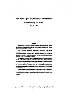
F IGURE 1. First iteration of Newton’s method to solve the nonlinear equation f (x) = (x − 1)2 (x + 1) = 0, given x0 = 2. P (xn , f (xn )). In the equation y = f (xn ) + f 0 (xn )(x − xn )
(2.1)
replace x by xn+1 and y by 0 to obtain the iteration equation of Newton’s method: xn+1 = xn −
f (xn ) ; with a given x0 . f 0 (xn )
(2.2)
This iteration equation can also be obtained using Taylor expansion. In Figure 1 the first iteration of Newton’s method (2.2) is displayed to calculate an approximation to the root α = 1 of f (x) = (x − 1)2 (x + 1) (in blue color) when x0 = 2 is used. In this case the tangent line (2.1) (in red color) at x = 2 is y = 7x − 11. So, if y = 0 then x1 = 11/7. When Newton’s method is used to approximate multiple roots, this does not work or at best, the order of convergence is reduced from quadratic to linear. To avoid this, Schr¨oder generates two new methods. Prior to presenting them, we need to define multiple roots and how to obtain from a given function with multiple roots, two related functions which have simple roots. Definition 2.1. α is a zero of f with multiplicity m > 0 if f (x) = (x − α)m g(x) where lim g(x) 6= 0.
x→α
In the case that m = 1, we say that α is a simple zero of f . p If α is a zero of f with multiplicity m, then α is a simple zero of F1 (x) = m f (x). α is also a simple zero of F2 (x) = ff0(x) (x) . When the multiplicity m of a root α is greater than one, then Newton’s method (2.2) has first order of convergence. To restore second method (2.2) p order convergence, Newton’s 1−m 1 [f (x)] m we obtain could be applied to the function F1 (x) = m f (x). Since F10 (x) = m xn+1 = xn − m
f (xn ) ; with a given x0 . f 0 (xn )
which is called the modified Newton’s method due to Schr¨oder [11].
(2.3)
Some Geometric Constructions of Two Variants of Newton’s Method to Solving Nonlinear Equations with Multiple Roots
When m is unknown, if we use in (2.2) the function F2 (x) = F20 (x)
derivative = 1 − Lf (x), where Lf (x) = iteration equation is obtained xn+1 = xn −
00
f (x)f (x) [f 0 (x)]2
f (x) f 0 (x)
17
(see [11]) and its
(see [4]-[6]), the following
f (xn ) 1 0 f (xn ) (1 − Lf (xn ))
(2.4)
which is called Newton’s method for multiple roots due to Schr¨oder [11]. In both methods (2.3) and (2.4), second order of convergence is achieved. 3. G EOMETRIC CONSTRUCTIONS WITH m KNOWN This section presents two geometric constructions to the modified Newton’s method. 3.1. Using straight line. Consider the straight line given by f 0 (xn ) (x − xn ) (3.5) m Iteration equation (2.3) can be obtained from this straight line whose slope is the m-th part of the derivative to the curve at the point whose abscissa is xn . The straight line (3.5) is secant to the curve y = f (x). This result is stated more precisely in the following theorem. y − f (xn ) =
Theorem 3.2. Let f : D ⊂ R → D be sufficiently differentiable in an open interval D and α a multiple zero of f with multiplicity m. Then the iteration (2.3) can be built from the curve defined by the equation (3.5) and this complies with the following two conditions: 0 n) y(xn ) = f (xn ) and y 0 (xn ) = f (x m . Proof. When evaluating x = xn in (3.5), y(xn ) = f (xn ) is obtained. On the other hand 0 0 n) n) deriving (3.5), y 0 = f (x is obtained and thus y 0 (xn ) = f (x m m . Finally using y = 0 and x = xn+1 in (3.5), we obtain (2.3). ¤ In Figure 2 the first iteration of the modified Newton’s method (2.3) is shown to calculate an approximation to the root α = 1 of f (x) = (x − 1)2 (x + 1) (in blue color) when x0 = 2 is used. In this case the secant line (3.5) in red color is y = 27 x − 4. So, if y = 0 then x1 = 8/7. 3.3. Using a polynomial of degree m. To obtain a curve that complies with the tangency conditions, begin with the straight line equation y = F1 (xn ) + F10 (xn )(x − xn ) which is tangent in x = xn to the curve whose equation is F1 (x) = the values of F1 (xn ) and F10 (xn ) in (3.6) we see that p m p f (xn )f 0 (xn ) m y= f (xn ) + (x − xn ) mf (xn ) √ Now, we proceed to substitute y by m y p m p f (xn )f 0 (xn ) √ m m y= f (xn ) + (x − xn ) mf (xn )
p
m
(3.6) f (x). Substituting
18
Carlos E. Cadenas R.
5 4 3 2 1 0 −1 0.5
α 1
x0
x1 1.5
2
2.5
F IGURE 2. First iteration of Modified Newton’s method to solve the nonlinear equation f (x) = (x − 1)2 (x + 1) = 0, given x0 = 2. Case: secant line y = 72 x − 4. It remains to confirm that this equation satisfies the conditions of tangency given in the following theorem: Theorem 3.4. Let α be a multiple zero of f with multiplicity m. Then the iteration (2.3) can be built from the curve defined by the equation µ ¶m f 0 (xn )(x − xn ) y = f (xn ) 1 + (3.7) mf (xn ) and complies with the following two conditions: y(xn ) = f (xn ) and y 0 (xn ) = f 0 (xn ) Proof. When evaluating x = xn in (3.7), y(xn ) = f (xn ) is obtained. If we replace x = xn in µ ¶m−1 f 0 (xn )(x − xn ) y 0 = f 0 (xn ) 1 + mf (xn ) then y 0 (xn ) = f 0 (xn ). Finally using y = 0 and x = xn+1 in (3.7) we obtain (2.3).
¤
Note that if m ∈ N then (3.7) is a polynomial of degree m. 28 16 2 In Figure 3 the parabola (in red color) P1 (x) = 49 12 x − 3 x + 3 is that obtained in the first iteration of the modified Newton’s method (2.3) when this is applied to f (x) = (x − 1)2 (x + 1) (in blue color) with x0 = 2. Observe that the intersection of P1 (x) with the axis x is in x1 = 8/7 and that the polynomial P1 is tangent to f at the point x = 2. 4. G EOMETRIC CONSTRUCTIONS WITH m UNKNOWN This section presents two geometric constructions of Newton’s method for multiple roots (2.4) which does not require prior knowledge of m.
Some Geometric Constructions of Two Variants of Newton’s Method to Solving Nonlinear Equations with Multiple Roots
19
5 4 3 2 1 0
α
−1 0.5
1
x0
x1 1.5
2
2.5
F IGURE 3. First iteration of Modified Newton’s method to solve the nonlinear equation f (x) = (x − 1)2 (x + 1) = 0, given x0 = 2. Case: 28 16 2 polynomial y = 49 12 x − 3 x + 3 . 4.1. Using straight line. The iteration equation (2.4) can be obtained from the straight line defined by the equation y = f (xn ) + f 0 (xn )[1 − Lf (xn )](x − xn )
(4.8)
The slope of this line is 1 − Lf (xn ) times the derivative of the curve at the point whose abscissa is xn . This implies that the straight line (4.8) is secant to the curve y = f (x). More precisely: Theorem 4.2. Let f : D ⊂ R → D be sufficiently differentiable in an open interval D and α a multiple zero of f with multiplicity m. Then the iteration (2.4) can be built from the curve defined by the equation (4.8) and this complies with the following two conditions: y(xn ) = f (xn ) and y 0 (xn ) = f 0 (xn )[1 − Lf (xn )]. Proof. When evaluating x = xn in (4.8) then y(xn ) = f (xn ) is obtained. On the other hand deriving (4.8) y 0 = f 0 (xn )[1 − Lf (xn )] is constant, so y 0 (xn ) = f 0 (xn )[1 − Lf (xn )]. Finally using y = 0 and x = xn+1 in (4.8), we obtain (2.4). ¤ In Figure 4 the first iteration of Newton’s method for multiple roots (2.4) is shown to approximate the root α = 1 of f (x) = (x − 1)2 (x + 1) (in blue color) when x0 = 2 is 17 used. In this case the secant line (4.8) in red color is y = 19 7 x − 7 in which y = 0 implies x1 = 17/19. 4.3. Using a rational function. To obtain a curve that complies with the tangency conditions begin by substituting in the equation f (xn ) 1 xn+1 = xn − 0 00 f (x n )f (xn ) f (xn ) 1 − 0 2 [f (xn )]
the value of y − f (xn ) for −f (xn ) and x for xn+1 (see [2]), giving x = xn +
y − f (xn ) f 0 (xn ) 1 +
1 (y−f (xn )f 00 (xn )) [f 0 (xn )]2
20
Carlos E. Cadenas R.
5 4 3 2 1 0 −1 0.5
x1
α
x0
1
1.5
2
2.5
F IGURE 4. First iteration of Newton’s method for multiple roots to solve the nonlinear equation f (x) = (x − 1)2 (x + 1) = 0, given x0 = 2. Case: 17 secant line y = 19 7 x− 7 . Here the following curve is obtained y = f (xn ) +
[f 0 (xn )]2 (x − xn ) 00 n ) − f (xn )(x − xn )
f 0 (x
(4.9)
It remains to confirm that this equation satisfies the conditions of tangency given in the following: Theorem 4.4. Let f : D ⊂ R → D sufficiently differentiable in an open interval D and α a multiple zero of f with multiplicity m. Then the iteration (2.4) can be built from the curve defined by the equation (4.9) which complies with the following two conditions: y(xn ) = f (xn ), y 0 (xn ) = f 0 (xn ) and y 00 (xn ) = 2f 00 (xn ). Proof. When evaluating x = xn in (4.9), y(xn ) = f (xn ) is obtained. As y0 =
[f 0 (xn )]3 [f 0 (xn ) − f 00 (xn )(x − xn )]2
and
2[f 0 (xn )]3 f 00 (xn ) 00 3 n ) − f (xn )(x − xn )] then y 0 (xn ) = f 0 (xn ) and y 00 (xn ) = 2f 00 (xn ). Finally, using y = 0 and x = xn+1 in (4.9) we obtain (2.4). ¤ y 00 =
[f 0 (x
In Figure 5 the first iteration of Newton’s method for multiple roots (2.4) is shown to calculate an approximation to the root α = 1 of f (x) = (x−1)2 (x+1) (in blue color) when 19x−17 x0 = 2 is used. In this case the tangent rational function (4.9) in x = 2 is y = 27−10x , which is represented in red color. So, if y = 0 then x1 = 17/19. 5. C ONCLUSION In this paper we have presented a straight line (3.5) and a curve (3.7) to obtain the iteration equation of the modified Newton’s method (2.3) when m ∈ N is known and (3.7) is a polynomial of degree m.
Some Geometric Constructions of Two Variants of Newton’s Method to Solving Nonlinear Equations with Multiple Roots
21
5 4 3 2 1
x1
0
α
−1 0.5
1
x0 1.5
2
2.5
F IGURE 5. First iteration of Newton’s method for multiple roots to solve the nonlinear equation f (x) = (x − 1)2 (x + 1) = 0, given x0 = 2. Case: 19x−17 tangent rational function y = 27−10x . We also presented when m is unknown, a straight line (4.8) and an equilateral hyperbola (4.9) to obtain the iteration equation (2.4). 6. ACKNOWLEDGMENTS The author is grateful to the editor and the referees for their valuable comments and suggestions. The author is also grateful to Professor Victor Griffin for his collaboration in the final writing. R EFERENCES [1] S. Amat, S. Busquier and J. M. Guti´errez, Geometric constructions of iterative functions to solve nonlinear equations, J. Comput. Appl. Math. 157, (2003) 197-205. [2] C. E. Cadenas, On several iterative methods of third order, based on Gander’s theorem for solving nonlinear equations and their geometric constructions, submited, (2017) [3] E. Hansen and M. Patrick, A family of root finding method, Numer. Math. 27, (1977) 257-269. [4] M. A. Hern´andez, An acceleration procedure of Whittaker method by means of the convexity, Univ. u Novom Sadu Zb. Rad. prirod. - Mat. Fak. Ser. Mat. 20, No. 1 (1990) 27-38. [5] M. A. Hern´andez. Newton-Raphson’s method and convexity, Zb. Rad. Prirod.-Mat. Fak. Ser. Mat. 22, No. 1 (1992) 159-166. [6] M. A. Hern´andez and M. A. Salanova, Indices of convexity and concavity, Application to Halley method. Appl Math Comput. 103, No. 1 (1999) 27-49. [7] A. Melman, Geometry and convergence of Euler’s and Halley’s methods, SIAM Rev. 39, No. 4 (1997) 728-735. [8] A. M. Ostrowski, Solution of equations and systems of equations, Prentice-Hall, Engle-wood Cliffs, NJ, USA, 1964. [9] A. M. Ostrowski, Solution of Equations in Euclidean and Banach Space, Academic Press, New York, 1973. [10] T. R. Scavo and J. B. Thoo, On the geometry of Halley’s method, Am Math Mon 102, (1995) 417-426. ¨ unendlichviele Algorithm zur Auffosung der Gleichungen, Math. Ann. 2, (1870) 317-365. [11] E. Schr¨oder, Uber [12] J. F. Traub, Iterative methods for resolution of equations, Prectice Hall, NJ 1964.