Boltzmann law of radiation. Stefan published further ..... However, the Admiralty had not planned a rescue mission in case of emergency. Franklin's ships.
Some historical notes on the Stefan problem. C. Vuik, Faculty of Faculty of Electrical Engineering, Mathematics and Computer Science, Delft University of Technology, Mekelweg 4, 2628 CD Delft. The Netherlands.
1
Introduction.
Nowadays a large class of problems - containing a free or moving boundary - are called Stefan problems (after J. Stefan, 1835-1893). The original Stefan problem treats the formation of ice in the polar seas. This paper gives some new information - which is not very well-known yet about the history of this problem. Stefan compares his mathematical results with measurements. He quotes Strachan (1879, 1880, 1882, 1885) as being the source of the measurements. However, he does not specify where the results given by Strachan come from. We shall show that these measurements were done during polar expeditions in order to find a North-West Passage. There is a much and rapidly growing interest in Stefan problems. This is illustrated by Table 1 where we give the average number of mathematical publications per year on the Stefan problem (see the bibliography given in [Cannon, 1984]). period average number Table 1
1931-40 0.1
1941-50 1.8
1951-60 4
1961-70 7.8
1971-80 23.3
1981-82 55
The average number of papers per year on the Stefan problem.
In the remainder of this section a short description is given about Stefan’s life and work. For more details we refer to [Gillespie, 1980]. In Section 2 we summarize Stefan’s research on ice formation. Some comparisons with measurements are given. The new insights are described in Section 3, where we show that the measurements were done during polar expeditions to discover a North-West Passage. Furthermore, some background information on these explorations is given. Section 4 contains some concluding remarks. Josef Stefan was born in St. Peter near Klagenfurt, Austria on 24 March 1835 and died a century ago on 7 January 1893. He enrolled at the University of Vienna in 1853. Stefan became a full professor of higher mathematics and physics at his alma mater in 1863 and three years later he was appointed director of the Institute for Experimental Physics, founded by Doppler in 1850. Stefan was a brilliant experimenter and a well-liked teacher. Stefan’s most important work deals with heat radiation (1879). He discovered that heat radiation is proportional to the fourth power of the absolute temperature. The theoretical deduction of this relationship was given by Boltzmann in 1884, leading to what is now known as the StefanBoltzmann law of radiation. Stefan published further experimental and theoretical works on the kinetic theory of heat: on heat conduction in fluids [Stefan, 1889a], on diffusion in fluids [Stefan, 1889b], on ice formation [Stefan, 1889c], and on evaporation [Stefan, 1889d]. In these papers Stefan describes mathematical models for physical problems, containing an interface of which the position changes in time. Since 1
Stefan gives the first detailed study of this type of problems, free or moving boundary problems are called Stefan problems. We note that the paper on ice formation in the polar seas [Stefan, 1889c] is reprinted as [Stefan, 1891]. Of the four papers published in 1889, this publication has drawn the most attention . As for the origin of the Stefan problem we note that a similar problem is already given in [Lam´e & Clapeyron, 1831]. They determined the thickness of a solid crust generated by the cooling of a liquid globe. Furthermore, the mathematical solution given in [Stefan, 1889c; p. 976, 977] was found by F. Neumann about 1860 and is known as the Neumann solution (see [Weber, 1901; p. 122]).
2
The Stefan problem.
2.1
The Stefan problem with a linear temperature profile.
We start with a description of the physical problem, which is investigated in [Stefan, 1891]. Consider a quantity of seawater which is cooled down to its freezing temperature. Suppose that at a certain time the temperature of the adjacent air decreases to α degrees below the freezing temperature of the seawater. Thereafter the temperature of the air does not change in time. Then ice formation begins at the interface between air and seawater. The resulting ice layer grows as a function of time. It is found that the thickness of the ice layer h is proportional to the square root of the elapsed time. This also follows from the mathematical model given in the following paragraph. Assume that the transport of heat through the ice is fast. This implies that the temperature in the ice has a linear profile. At the air-ice interface the temperature is equal to α degrees below the freezing temperature, whereas at the ice-water interface it is equal to the freezing temperature. These assumptions imply that the heat removed from the ice during a time dt is equal to Kα h .dt, where K is the heat-conduction coefficient of ice. If an amount dh of seawater changes to ice, then it produces an amount of heat equal to λσdh, where λ is the latent heat and σ the specific mass of ice. This leads to the following differential equation λσdh =
Kα dt, h
(1)
with solution given by
2Kα t. (2) λσ Stefan shows that the assumption of a linear temperature profile in the ice is reasonable, because the specific heat of ice (c=0.5) is much smaller than the latent heat (λ = 79). Furthermore, he gives some error estimates [Stefan, 1891; p. 271]. h2 (t) =
Stefan noted that the physical situation is much more complicated. Firstly, the temperature of the air is not constant. The temperature of the air starts at the freezing temperature, then it decreases to a minimum value and then it increases again to the freezing temperature. Secondly, due to this temperature variation of the air the linear temperature profile in the ice is lost, because it takes time to change the temperature in the ice, especially when the thickness of the ice layer becomes large. In Figure 1 this phenomenon is illustrated for the measurements done at the second ”Deutsche Nordpohlfahrt” in the years 1869-1870 [Stefan, 1891; p. 271- 273]. The measurements done on 11 November and 24 November 1869 can be reasonably approximated by a straight line. On 18 February 1870 the measurements show a considerable deviation below 40 inches, whereas on 21 May 1870 the heat moves into the opposite direction from the air into the ice. Supposing that the temperature of the air is a function of t: α(t) degrees below the freezing temperature, equation (2) leads to 2
2K h (t) = λσ 2
Z
t
α(τ )dτ.
(3)
0
A difficulty was that in 1891 the exact value of K, the heat conduction coefficient of ice was unknown. In [Stefan, 1891; p. 279] different values of K are given: K = 0.0057 after Neumann, K = 0.00223 after Forber and K = 0.005 after Mitchell. This motivated Stefan to approximate K from his experiments: K = 0.0042. A more recent value of K can be obtained from [Carslaw & Jaeger, 1950; p. 382] where K is equal to 0.0053 (in C.G.S. units and 0 C). They note that the value of K for non-metals is to be regarded as rough average values only, as there may be large differences between the thermal conductivities of different samples of the same substance. Transforming the value K = 0.0042 to the appropriate units, we obtain from (3) the following expression: Z t 2 h (t) = 0.869 α(τ )dτ (4) 0
where h is measured in inches, α in degrees Fahrenheit and t in days. Since the physical constant K is unknown, Stefan comparesR the measurements with his thet ory in the following way: he defined the quotient Q = h2 (t)/ 0 α(τ )dτ and calculated Q for all measurements. It appeared that there are only small differences between the calculated values of Q. The value 0.869 is the average. In this paragraph we use another comparison. We suppose that Q = 0.869 is the correct value and use the measurements done in the Gulf of Boothia in the winter of 1831-1832 (Table 2) [Stefan, 1891; p. 274]. We suppose that the ice layer is formed on 1 October 1831; Stefan [Stefan, 1891; p. 274] noted that in general the starting time of the ice formation is not given. The freezing temperature of seawater is equal to 28 0 Fahrenheit. We apR 31 R 61 proximate 0 α(τ )dτ by 31.(28-8.9), 0 α(τ )dτ by 31.(28-8.9) + 30.(28+1.2) etc. The resulting predictions and measurements are given in Figure 2. Note that although the predictions are based on crude measurements (the mean temperature of the air should be known every day), there is a good correspondence between the predictions and the measurements. In Figure 3 we see that the relation between the thickness of the ice and the cold-sum looks like the graph of a square root function, which is predicted by formula (4). Date 31 October 1831 30 November 1831 31 December 1831 3 February 1832 31 March 1832
Thickness of the ice 19 inch 33 inch 48 inch 60 inch 84 inch
Mean temperature of the air 8.9 0 F -1.2 0 F -24.0 0 F -27.6 0 F -33.0 0 F
Table 2. Measurements at the Gulf of Boothia.
Other comparisons given in [Stefan, 1891] show that the differences between predictions and measurements can be larger. Stefan gives some possible physical explanations [Stefan, 1891; p. 278]: - initially snow can isolate the ice so that the heat transport to the air is prohibited, or - there is a flow of warm water so that the increase of the thickness of the ice layer is much less than expected. It enhanced the credibility of Stefan’s work that he also gives measurements which show a not so good correspondence between theory and practice.
3
2.2
The Stefan problem with a general temperature profile.
We consider the second model described in [Stefan, 1891; p. 279-280]. In this model the instationar transport of heat in the ice is taken into account. In the following the difference of the freezing temperature and the temperature of the ice is denoted by u(x, t) (note that u(x, t) ≥ 0). In the ice layer the temperature difference satisfies the following partial differential equation: K ∂ 2 u(x, t) ∂u(x, t) = , ∂t cσ ∂x2 As initial condition it is supposed that
0 < x < h(t),
0 < t.
h(0) = 0.
(5)
(6)
At the air-ice interface the temperature is a given function of t u(0, t) = f (t),
(7)
whereas at the ice-water interface the temperature is equal to the freezing temperature u(h(t), t) = 0.
(8)
Another condition (comparable to equation (1)) at the ice-water interface follows from the heat balance and is given by: ∂u dh(t) = −K (h(t), t), 0 < t. (9) λσ dt ∂x Nowadays the equations (5) to (9) are considered to be the original Stefan problem. Taking f (t) = α, t > 0, the following solution is given [Stefan, 1891; p. 281]: r K t, h(t) = 2µ cσ Z µ Z µ 2 2 e−z dz/ e−z dz, u(x, t) = α x √ Kt 0 2
cσ
where µ is the solution of the following transcendental equation: Z µ 2 2 µc µeµ e−z dz = . 2λ 0 The results given in Section 2.1 can be seen as a reasonable approximation of the solution given above. For a more general problem, such that f (t) is not constant, Stefan gives some further ideas to obtain the solution, and calculates some approximations [Stefan, 1891; p. 283-286]. However, for this problem he was not able to give an explicit solution.
3
The origin of the measurements.
We now come to the central theme of this paper: what is the origin of the measurements reported in [Stefan, 1891]? Stefan quotes [Strachan, 1879, 1880, 1882, 1885] as his source. In the preface of [Strachan, 1879] the aim of the work is stated as: to collect and discuss the meteorological observations of British Expeditions to the arctic regions. In [Strachan, 1879] the results obtained from landstations are discussed, whereas [Strachan, 1880, 1882, 1885] contain results obtained from 4
ships, either frozen up in winter quarters, or drifting with the ice. Furthermore, it appears from Strachan’s work that all expeditions tried to find a North-West Passage. In Table 3 we specify the place and time of the measurements as given in [Stefan, 1891]. Some extra information obtained from Strachan is summarized in Table 4. Number
Place
Time
1. 2. 3. 4. 5. 6. 7. 8.
Gulf of Boothia Assistance Bay Port Bowen Walker Bay Cambridge Bay Camden Bay Princess Royal Islands Mercy Bay
1831-1832 1850-1851 1824-1825 1851-1852 1852-1853 1853-1854 1850-1851 1851-1852
Strachan part page 2 48 2 153 3 312 3 379 3 391 3 403 4 414 4 428
Table 3 Place and time of the measurements.
In the following subsections we give some more details, based mainly on the material given in [Lehane, 1982]. In Subsection 3.1 motivations for these expeditions are given and the first expedition is described. It follows from Table 3 and Strachan, that there is a peak in the number of measurements around 1850. In Subsection 3.2 we shall give the cause of this peak and conclude with some details on the journey of Robert McClure. Number 1. 2. 3. 4. 5. 6. 7. 8.
Western Longitude 90 95 89 117 105 145 117 117
Northern Latitude 70 75 73 71 69 71 72 75
Country
Explorer
Ships
Canada Canada Canada Canada Canada U.S.A. Canada Canada
John Ross William Penny William Parry Richard Collinson ” ” Robert McClure ”
”Victory” ”Lady Franklin” H.M.S. ”Hecla” & ”Fury” H.M.S. ”Enterprise” ” ” H.M.S. ”Investigator” ”
Table 4 Coordinates and explorers connected with the measurements.
3.1
The quest for a North-West Passage.
The quest for a North-West Passage from the Atlantic to the Pacific started five years after Columbus discovered America. In 1497 John Cabot (Giovanni Caboto, 1425-1498) sailed from England in a north-western direction in order to find a sea-route to the Far East. He arrived in Newfoundland (New Found Land), and assumed that he was in the neighbourhood of China. His wrong assumption was influenced by the inaccurate approximation of the circumference of the equator, 29,000 km after Ptolemaeus, instead of 40,000 km. His son Sebastian Cabot (Sebastiano Caboto, 1472-1557) detected this error during his own explorations. He was the first to suggest a North-West Passage through the new continent. Many explorers followed this suggestion. In the course of years the motivation for this quest changed significantly. Around 1600 there was a severe competition between British and Dutch East-Indian Companies to transport the treasures of the Far East to Europe. Both companies tried to discover the North-West Passage in order to obtain faster sea routes.
5
In England the interest for the North-West Passage revived from 1770. The reason is that if England discovered this route, then it would be easy to control or to obtain Canada. Furthermore, a fast route to the Pacific would be very important in case of a confrontation with Spain. From the explorations done in this period it was concluded that the Passage cannot be used for commercial purposes. The reason is that the route is far north, so it can only be used a small part of the year, and the ice formation in the polar seas makes it a dangerous route. After the Napoleonic wars the quest was continued. However, the main motivations in this period were: the challenge to find the Passage, and the fact that the scientific community was anxious to obtain more and better information about the arctic regions. In this period John Ross (1777-1856) is one of the main explorers. In 1818 he prepared and carried out an exploration of Baffin Bay. He entered Lancaster Sound in Baffin Bay, but due to a mirage concluded that the sound was closed by mountains. In 1819 he returned to England without losing a person. He had collected many scientific results: charts, compass-bearings, measurements of the specific mass and the temperature of sea water etc. In 1819 William Parry (1790-1855), a member of the expedition of 1818, showed the conclusion of Ross to be wrong. He sailed through Lancaster Sound. This was an important step in the discovery of the North-West Passage. In 1829 John Ross prepared another expedition to the polar seas. He wanted to correct his error and thought that Prince Regent Inlet was the missing link in the Passage. His wrong conclusion of 1818 was the reason that he did not obtain money from the Admiralty. His rich friend Felix Booth donated 18,000 pounds. This together with 3000 pounds of his own were sufficient to finance the exploration. In 1829 he was trapped in the ice of Prince Regent Inlet. This place is mentioned after his financier: the Gulf of Boothia. During winter they did scientific observations. Some of these are the discovery of the magnetic North Pole, the measurements of the temperature of the air and the thickness of the ice layer. These measurements were used in [Stefan, 1891], see Table 3 and 4. The background of the measurements also explains the fact that the starting time of the ice formation is unknown [Stefan, 1891; p. 274], because these measurements were not planned but were done by accident. After four winterings the people of this expedition left their ship, and escaped with small boats to Lancaster Sound. They were picked up by another ship and returned to England in 1833.
3.2
The last expedition of John Franklin.
The peak in the measurements around 1850, which we mentioned above, was caused by a number of rescue expeditions, which looked for the lost expedition of the British Captain Sir John Franklin. John Franklin (1786-1847) departed on 15 May, 1845 with two ships to discover the last missing links of the North-West Passage. They had sufficient victuals on board for a voyage of three years. However, the Admiralty had not planned a rescue mission in case of emergency. Franklin’s ships were seen on 16 June 1845 in the vicinity of Lancaster Sound. Thereafter these explorers were never seen again. In retrospect, the voyage of Franklin can be reconstructed. He sailed to Lancaster Sound. Near Cape Walker the passage was closed by pack ice. So they sailed to the north, around Cornwallis Island, and spent the winter at Beechey Island. Here, three of Franklin’s men died and were buried on the spot. In 1846 they discovered and entered Peel Sound. In this sea-route they were again trapped in the ice. Franklin died on 11 June 1847. In 1848 the remainder of his crew left the ships and walked to the south. Nobody survived this attempt to escape. Since Franklin’s expedition did not return, the Admiralty sent several rescue expeditions. In 6
1850 for instance, twelve ships were in the arctic regions, looking for survivors. A reward of 20.000 pounds was promised to the expedition which would find Franklin and his crew. Some commanders were more interested in finding the North-West Passage themselves, than to find an explorer who had failed in such an attempt. Many of these expeditions were also trapped in the polar ice. This explains the peak in the measurements around 1850 as noted above. These expeditions have found the missing links of the North-West Passage. One of these rescue missions was led by Robert McClure (1807-1873). He departed on 10 January 1850 for a voyage round Cape Horn to the Pacific Ocean. From there he sailed to Bering Strait in order to look for Franklin’s expedition along the north Canadian coastline. On 11 September 1850 the ship was trapped in the ice in Melville Sound, near the Princess Royal Islands. In July 1851 the ship got loose from the ice. McClure sailed around Banks Island to the north. However, they got trapped again in Mercy Bay, where they remained for two winters. On 6 April 1853 members of an expedition from the Atlantic Ocean arrived at McClure. This was the first time in history that an expedition of the Pacific met an expedition coming from the Atlantic. McClure’s crew walked 200 miles across the ice of Melville Sound to Dealy Island. From there they departed to England. After arriving McClure was made a hero and honoured for achieving a passage through the Canadian polar seas. However, he did not made the voyage on the same ship. Thereafter no major expeditions were sent, until the Norwegian Roald Amundsen (1872-1928) crossed the North-West Passage. He made use of the results obtained by preceding expeditions. He departed on 16 June 1903 with a crew of 6 men on the steam-yacht Gj¨ oa of 47 tons. He wintered in 1904 and 1905 in Rae Strait and completed the passage in 1906. For nearly one and a half century it has remained unclear why the 129 men of the Franklin expedition perished in the arctic region. Recent scientific research has shown that technological improvements had been fatal to them [Beattie & Geiger, 1987]. Owen Beattie discovered some bones of one of Franklin’s men and an Inuit skeleton at Booth Point on King William Island in 1981. It appeared that the European had died from scurvy. From an analysis of the bones in his laboratory Beattie noted that the bones of Inuit contained 30 ppm lead, whereas the bones of the European contained 230 ppm lead. So this member of Franklin’s crew also suffered from an acute lead poisoning. It is possible that the lead had been built up over a long period. In order to verify that lead poisoning was the cause of the death of Franklin’s men, Beattie carried out an excavation of Franklin’s men, buried at Beechey Island (1984). Hair of the excavated corpses contained 600 ppm lead. The mystery of the loss of the Franklin expedition was solved. The explorers died from lead poisoning. The poisoning was caused by canned food, a new technology. Franklin was the first to take canned food on a polar expedition. The cans were made in London. After filling, the cans were closed with solder tin, which consists of 90% lead and 10% tin. Apparently this closure was done uncarefully, so that the food contained too much lead, causing the death of the explorers.
4
Concluding remarks.
In 1889 Stefan had written four papers on free boundary problems. The paper on ice formation in the polar seas was reprinted in 1891 and has drawn the most attention of the scientific community. In this paper we have shown that the physical results used in [Stefan, 1891] were obtained at quests for a North-West Passage. The attention drawn by [Stefan, 1891] is possibly related to the fact that in Stefan’s time the North-West Passage had not been achieved with one ship. Furthermore, Stefan’s paper appeared some years after a peak in expeditions to the arctic around 1850. Since the mathematical model on ice formation given by Stefan is easily solved and gives reasonable results, it could have been useful for polar expeditions. After 1815 the motivation to perform the expeditions was mainly to obtain more and better 7
information about the arctic regions for the scientific community. This aim was achieved, and by way of Stefan’s paper the expeditions have had a considerable impact on some parts of scientific research, see for instance Table 1 in the introduction. Note that nowadays the formation of ice in the polar regions is again an important topic of research, related to a possibly increasing trend of temperature of the global atmosphere.
References 1. O. Beattie & J. Geiger, Frozen in time: the fate of the Franklin expedition, Bloomsbury, London, (1987). 2. J.R. Cannon, The one-dimensional heat equation, Addison Wesley, Reading, (1984). 3. H.S. Carslaw & J.C. Jaeger, Conduction of heat in solids, Oxford University Press, Oxford, 1950. 4. C.C. Gillespie (editor), Dictionary of scientific biography, Volume 13, p. 10-11, Charles Scribner’s Sons, New York, (1980). 5. G. Lam´e, B.P. Clapeyron, M´emoire sur la solidification par refroidissement d’un globe solide, Ann. Chem. Phys. 47, 250-256, (1831). 6. B. Lehane, De Noordwestelijke doorvaart, Serie: De zeevaart, Time Life boeken, Amsterdam, (1982). 7. J. Stefan (1889a), ¨ ¨ Uber einige Probleme der Theorie der W¨ armeleitung, Sitzungsberichte der Osterreichischen Akademie der Wissenschaften Mathematisch-Naturwissenschaftliche Klasse, Abteilung 2, Mathematik, Astronomie, Physik, Meteorologie und Technik, 98, 473-484, (1889). 8. J. Stefan (1889b ), ¨ ¨ Uber die Diffusion von Sauren und Basen gegen einander, Sitzungsberichte der Osterreichischen Akademie der Wissenschaften Mathematisch-Naturwissenschaftliche Klasse, Abteilung 2, Mathematik, Astronomie, Physik, Meteorologie und Technik, 98, 616-634, (1889). 9. J. Stefan (1889c), ¨ Uber die Theorie der Eisbildung, insbesondere u ¨ber die Eisbildung im Polarmeere, Sitzungs¨ berichte der Osterreichischen Akademie der Wissenschaften Mathematisch-Naturwissenschaftliche Klasse, Abteilung 2, Mathematik, Astronomie, Physik, Meteorologie und Technik, 98, 965-983, (1889). 10. J. Stefan (1889d), ¨ Uber die Verdampfung und die Aufl¨ osung als Vorgange der Diffusion, Sitzungsberichte ¨ der Osterreichischen Akademie der Wissenschaften Mathematisch-Naturwissenschaftliche Klasse, Abteilung 2, Mathematik, Astronomie, Physik, Meteorologie und Technik, 98, 14181442, (1889). 11. J. Stefan, ¨ Uber die Theorie der Eisbildung, insbesondere u ¨ber die Eisbildung im Polarmeere, Annalen der Physik und Chemie, 42, 269-286, (1891). 12. R. Strachan, Contributions to our knowledge of the meteorology of the arctic regions, Part 1, London, 1879. 8
13. R. Strachan, Contributions to our knowledge of the meteorology of the arctic regions, Part 2, London, 1880. 14. R. Strachan, Contributions to our knowledge of the meteorology of the arctic regions, Part 3, London, 1882. 15. R. Strachan, Contributions to our knowledge of the meteorology of the arctic regions, Part 4, London, 1885. 16 H. Weber, Die partiellen Differential-Gleichungen der mathematischen Physik II, Vieweg, Braunschweig, (1901).
0
-10
Depth in inch
-20
-30
-40
1869 -- 11 November .. 24 November1869
-50
_ 18 February 1870 1870
-. 21 May -60 -25
-20
-15 -10 Temperature in Reaumur
-5
0
Figure 1: Measurements from the second ”Deutsche Nordpohlfahrt”
9
90
Thickness of the ice-layer in inches
80 70 60 50 40 30 20 _ calculations * measurements
10 0 0
20
40
60 80 100 120 Days from 1 October, 1831
140
160
180
Figure 2: Measurements at the Gulf of Boothia compared with calculations
90
Thickness of the ice-layer in inches
80 70 60 50 40 30 20 _ calculations * measurements
10 0 0
1000
2000
3000 4000 5000 6000 7000 Cold-sum (days*temperature)
8000
9000
Figure 3: Measurements at the Gulf of Boothia compared with calculations
10