3 James D. Foley, Andries van Dam, Steven K. Feiner, and John F. Hughes, Computer Graph- ... 4 William M. Newman and Robert F. Sproull, Principles of Interactive ... 11 Mike Cyrus and Jay Beck, ''Generalized Two- and Three-Dimensional ...
Some Improvements to a Parametric Line Clipping Algorithm You-Dong Liang†, Brian A. Barsky, Mel Slater‡
Computer Science Division University of California Berkeley, California 94720 U.S.A.
This paper presents an improved version of our earlier1, 2 parametric line clipping algorithm. There are two types of improvements. The first involves an initial trivial reject test based only on comparisons, and the second is the addition of a test to avoid unnecessary computation when the result will not affect the parametric value of the intersection point. For each dimension, the mathematics are derived along with geometrical interpretations and the algorithm is designed. Finally, a performance test is conducted. Both the original and improved versions of our algorithm are compared to the traditional SutherlandCohen3, 4 clipping algorithm. 0. Introduction Clipping is a basic and important problem in computer graphics. It is the process of removing that portion of an image that lies outside a region called the clip window or visible region.5, 6 One way to classify clipping algorithms is according to the type of h hhhhhhhhhhhhhh
† Permanent address: Department of Mathematics, Zhejiang University, Hangzhou, Zhejiang People’s Republic of China ‡ Permanent address: Department of Computer Science, QMW University of London, Mile End Road, London E1 4NS, U.K. 1 You-Dong Liang and Brian A. Barsky, ‘‘A New Concept and Method for Line Clipping,’’
ACM Transactions on Graphics, Vol. 3, No. 1, January, 1984, pp. 1-22. 2 You-Dong Liang and Brian A. Barsky, ‘‘Introducing A New Technique for Line Clipping,’’ pp. 548-559 in Proceedings of the International Conference on Engineering and Computer Graphics, Beijing, 27 August - 1 September 1984. Also in Journal of Zhejiang University Special Issue on Computational Geometry, 1984, pp.1-12. 3 James D. Foley, Andries van Dam, Steven K. Feiner, and John F. Hughes, Computer Graphics: Principles and Practice, Addison-Wesley Publishing Company, 1990. Second Edition. 4 William M. Newman and Robert F. Sproull, Principles of Interactive Computer Graphics, McGraw-Hill, 1979. Second edition. 5 James D. Foley, Andries van Dam, Steven K. Feiner, and John F. Hughes, Computer Graphics: Principles and Practice, Addison-Wesley Publishing Company, 1990. Second Edition. 6 William M. Newman and Robert F. Sproull, Principles of Interactive Computer Graphics, McGraw-Hill, 1979. Second edition.
-2primitive upon which they operate; the type of clipping to be considered in this paper is line clipping. In the early time of computer graphics, the Sutherland/Cohen7, 8 line clipping algorithm and its coding technique was in common use. In 1984, we proposed a family of efficient line clipping algorithms that are based on a strict mathematical form.9, 10 Our line clipping algorithm employed a parametric representation of the line segment to be clipped, used minimum and maximum calculations to determine the parametric values corresponding to the endpoints of the visible line segment, and developed several new definitions for trivial reject to speed up the approach. A similar approach was independently adopted by Cyrus and Beck11 although that work did not develop the trivial reject cases that are so important for efficiency. The method for line clipping that we developed describes clipping in an exact and mathematical form. The basic ideas form the foundation for a family of algorithms for two-, three-, and four- (homogeneous coordinates) dimensional line clipping. One of the features of our algorithm is that it is independent of dimension. The identical coded procedure can be used for clipping in any dimension. The applicability of this algorithm for different dimensions only requires a different calling sequence for this procedure. This feature is both theoretically interesting and practically convenient. For this reason, the computation times for our algorithm are fairly constant over the different dimensions. At SIGGRAPH’87, Nicholl, Lee, and Nicholl12 presented a very efficient twodimensional line clipping algorithm that is based on a case-by-case approach and which improved upon the existing line clipping algorithms. However, their algorithm is only applicable in two dimensions. In our algorithm, the line segment to be clipped is mapped into a parametric representation. >From this, a set of conditions is derived that describes the interior of the clipping region. Observing that these conditions are all of similar form, they are rewritten such that the solution to the clipping problem is reduced to a simple max/min expression. h hhhhhhhhhhhhhh
7
James D. Foley, Andries van Dam, Steven K. Feiner, and John F. Hughes, Computer Graphics: Principles and Practice, Addison-Wesley Publishing Company, 1990. Second Edition. 8 William M. Newman and Robert F. Sproull, Principles of Interactive Computer Graphics, McGraw-Hill, 1979. Second edition. 9 You-Dong Liang and Brian A. Barsky, ‘‘A New Concept and Method for Line Clipping,’’ ACM Transactions on Graphics, Vol. 3, No. 1, January, 1984, pp. 1-22. 10 You-Dong Liang and Brian A. Barsky, ‘‘Introducing A New Technique for Line Clipping,’’ pp. 548-559 in Proceedings of the International Conference on Engineering and Computer Graphics, Beijing, 27 August - 1 September 1984. Also in Journal of Zhejiang University Special Issue on Computational Geometry, 1984, pp.1-12. 11 Mike Cyrus and Jay Beck, ‘‘Generalized Two- and Three-Dimensional Clipping,’’ Computers and Graphics, Vol. 3, No. 1, 1978, pp. 23-28. 12 Tina M. Nicholl, D. T. Lee, and Robin A. Nicholl, ‘‘An Efficient New Algorithm for 2-D Line Clipping: Its Development and Analysis,’’ pp. 253-262 in SIGGRAPH ’87 Conference Proceedings, ACM, Anaheim, July 27-31, 1987.
-3Another advantage of our algorithm is that line segments that are invisible are quickly rejected. In addition, although the three-dimensional and homogeneous coordinate algorithms are presented for perspective viewing volumes, it should be noted that it is equally appropriate for non-perspective viewing volumes, and more generally, for any convex visible region. Furthermore, the structure of the algorithm is such that the conditions describing the interior of the clipping region are all of similar form; consequently, these visibility calculations could be processed in parallel. In this paper, we describe an improved version of this algorithm. There are three types of improvements. First, we introduce an initial test for trivial reject, that is, based only on comparisons between the line endpoints and the clipping boundaries. Second, the original algorithm employed two different kinds of tests to accomplish subsequent trivial rejects; in the improved version, we add a third type of test for trivial reject. Third, tests are added so as to avoid unnecessary computation when the result will not affect the parametric value of the intersection point. For each dimension, the mathematics are discussed and the algorithm is designed, and then a performance test is conducted. Both the original and improved versions of our algorithm are compared to the traditional Sutherland-Cohen13, 14 clipping algorithm. Using randomly generated data, the original version of our algorithm showed a 25% to 62% improvement compared to the Sutherland-Cohen algorithm and the improved version of our algorithm had a 46% to 68% improvement over the Sutherland-Cohen algorithm. 1. Setting up the Problem in Two, Three, and Four Dimensions In two-dimensional clipping, lines are clipped against a two-dimensional region called the clip window (Figure 1-1). In particular, let the equations of the boundary lines be x = x left x = x right y = y bottom
(1.1)
y = y top representing the left, right, bottom, and top boundaries, respectively. Using this notation, a two-dimensional point ( x , y ) is inside the window if and only if x left ≤ x ≤ x right y bottom ≤ y ≤ y top h hhhhhhhhhhhhhh
13
James D. Foley, Andries van Dam, Steven K. Feiner, and John F. Hughes, Computer Graphics: Principles and Practice, Addison-Wesley Publishing Company, 1990. Second Edition. 14 William M. Newman and Robert F. Sproull, Principles of Interactive Computer Graphics, McGraw-Hill, 1979. Second edition.
(1.2)
-4-
Figure 1-1: The interior of the clip window. For three-dimensional clipping, lines are clipped against a viewing pyramid. In this case, the coordinate system is transformed to a right-pyramid coordinate system where the viewing volume is a right pyramid, as shown in Figure 1-2a. The equations of the four bounding planes of the right pyramid are: z = −x z =x z = −y z =y
(1.3)
representing the left, right, bottom, and top bounding planes, respectively. >From this, a three-dimensional point ( x , y , z ) is inside the viewing volume if and only if −z ≤ x ≤ z (1.4) −z ≤ y ≤ z and z ≥ 0 is implied. This can be extended to cover the case of a finite viewing volume. Here, the viewing pyramid is truncated by hither and yon clipping planes to form a frustum of vision, as shown in Figure 1-2b. Note that the location of these planes is completely independent of the position of the picture plane. This requires the addition of constraints for z. If the hither and yon clipping planes are z =h and z =f, respectively, then these constraints are: h ≤z ≤ f
(1.5)
In the case of four-dimensional clipping with perspective depth transformation, a homogeneous coordinate system is employed. Clipping is performed after the application of the perspective transformation, but prior to the perspective depth division. This is called "clipping in homogeneous coordinates". The clipping limits in this formulation are: −w ≤ x ≤ w −w ≤ y ≤ w (1.6) 0≤z ≤w
-5-
Figure 1-2: Viewing volumes for three-dimensional clipping. (a) The right pyramid viewing volume (left). (b) The frustum of vision (right). 2. Two-Dimensional Line Clipping Algorithm 2.1. Explanation Recall the two-dimensional clipping limits given by inequalities (1.2): x left ≤ x ≤ x right (2.1)
y bottom ≤ y ≤ y top
The line segment to be clipped is mapped into a parametric representation as follows. Recall that our notation for the endpoints of the line segment is V0 and V1 with coordinates (x 0 , y 0 ) and (x 1 , y 1 ), respectively. Then the parametric representation of the line is given by x = x 0 + ∆x t (2.2) y = y + ∆y t 0
where ∆x = x 1 − x 0 (2.3)
∆y = y 1 − y 0
The parametric values corresponding to V0 and V1 are t =0 and t =1, respectively. As t varies from t =0 to t =1, the line segment V0 V1 is traced out from V0 to V1 ; allowing − ∞ < t < ∞ generates the line of infinite extent. Substituting the parametric representation given by equations (2.2) and (2.3) into inequalities (2.1) yields the following conditions for the part of the extended line that is inside the interior of the clip window: −∆x t ≤ x 0 − x left and ∆x t ≤ x right − x 0 (2.4) −∆y t ≤ y − y and ∆y t ≤ y − y 0
bottom
top
0
-6Note that these conditions (2.4) are inequalities describing the interior of the clip window rather than equations defining its boundary. Observe that inequalities (2.4) are all of similar form; thus, they can be rewritten as pi t ≤ qi for i=1, 2, 3, 4
(2.5)
where the following notation is used: p 1 = −∆x q 1 = x 0 − x left p 2 = ∆x
q 2 = x right − x 0
p 3 = −∆y q 3 = y 0 − y bottom p 4 = ∆y
(2.6)
q 4 = y top − y 0
To establish a geometrical interpretation of these four inequalities, extend each of the four boundary line segments of the clip window to be a line of infinite extent. Each of these lines divides the plane into two regions; we define the visible side to be that side on which the clip window lies, as shown in Figure 2-1.
Figure 2-1: The visible side of a boundary line. In this way, the clip window can be defined as that region that is on the visible side of all the boundary lines. From this, it can be seen that each of the inequalities (2.5) corresponds to one of these boundary lines (left, right, bottom, and top, respectively), and describes its visible side. In the improved version of the algorithm, a trivial reject test is performed prior to any other computation. The two endpoints of the line segment are checked against each boundary line in turn to see if they both lie on the invisible side of the boundary line. If they do, for any boundary, then the line segment is trivially rejected as invisible, and no further computation needs to be performed. If the line segment is not trivially rejected against any boundary, then the remainder of the algorithm is based on the following analysis. Extend V0 V1 to be a line of infinite extent. Then each inequality provides the range of values of the parameter t for which this extended line is on the visible side of the corresponding boundary line. Furthermore, the particular parametric value for the point of intersection is t=qi /pi . Also, the sign of qi indicates on which side of the corresponding boundary line the point V0 lies. Specifically, if qi ≥ 0, then V0 is on the visible side of the boundary line (inclusive), and if qi < 0, then V0 is on the invisible side. Considering the pi ’s in equation (2.6), it is clear that each can be negative, positive, or zero. If pi is negative, the i’th inequality becomes t ≥ qi /pi
(2.7)
Observing that the range of parametric values for which the extended line is on the visible side of the corresponding boundary line is at a minimum at the point of intersection, hhhhh → the direction defined by V0 V1 is from the invisible side to the visible side of the
-7boundary line. Analogously, if pi is positive, the i’th inequality becomes t ≤ qi /pi
(2.8)
Since the parametric range is at a maximum at the point of intersection, the direction hhhhh → defined by V0 V1 must be from the visible side to the invisible side of the corresponding boundary line. Finally, if pi is zero, the i’th inequality becomes 0 ≤ qi
(2.9)
Note that this is now independent of t. Thus, the inequality is satisfied for all t if qi ≥ 0, and there is no solution if qi < 0. Geometrically, if pi is zero, there is no point of intersection of the extended line with the corresponding boundary line; rather, they are parallel. Furthermore, if qi ≥ 0, then in this case the entire extended line is on the visible side of the boundary line (inclusive); if qi < 0, then it is entirely on the invisible side of the line. In the former case, there may or may not be a visible segment depending on where V0 and V1 lie on the extended line. However, the latter case cannot have a visible segment since the extended line lies outside the visible region and hence this is a trivial reject case. All these cases are summarized in the flowchart shown in Figure 2-2.
Figure 2-2: Flowchart showing the geometrical interpretations for the pi and qi values. Now, the intersection of the four inequalities gives the range of values of the parameter t for which the extended line is inside the clip window. However, the line segment to be clipped (V0 V1 ) is only part of the extended line and is described by 0 ≤ t ≤ 1. Hence, the solution to the two-dimensional clipping problem is equivalent to the inequalities (2.5) under the condition 0 ≤ t ≤ 1.
-8Solving these inequalities is actually a max/min problem, which can be seen as follows. Recall that t ≥ qi /pi for all i such that pi 0, i = 1, 2, 3, 4}∪{1})
(2.11)
Finally, if pi =0 in the i’th inequality for some i, then there are two possibilities. If qi ≥ 0, then there is no useful information to be gleaned from this inequality, and this inequality can be discarded. If qi < 0, then this is a trivial reject case, and the clipping problem is solved with no further computation needed. The righthand sides of equations (2.10) and (2.11) are the values of the parameter t corresponding to the beginning and end of the visible segment, respectively (assuming there is a visible segment). Denoting these parametric values as t 0 and t 1 , t 0 = max ({qi /pi c pi 0, i = 1, 2, 3, 4} {1}) 1
i
i
∪
i
If there is a visible segment, it corresponds to the parametric interval t0 ≤ t ≤ t1
(2.13)
Hence, a necessary condition for a line segment to be at least partially visible is t0 ≤ t1
(2.14)
This is not a sufficient condition because it ignores the possibility of a trivial reject due to pi =0 with qi t 1 , then this is another reject case. The algorithm checks if pi =0 with qi t 1 , in which case the line segment is immediately rejected without further computation. The algorithm initializes t 0 and t 1 to 0 and 1, respectively. Then each boundary line is considered successively. In the case of entering the visible region (pi z1)) or ((x0 < -z0) and (x1 < -z1)) or ((y0 < -z0) and (y1 < -z1)) or ((z0 < h) and (z1 < h)) or ((z0 > f) and (z1 > f))) then begin (* trivial reject *) visible := false; goto 1; end; (* trivial reject *) begin (* not trivial reject *) visible := false; t0 := 0; t1 := 1; deltax := x1 - x0; deltaw := w1 - w0; if clipt (- deltax - deltaw, x0 + w0, t0, t1) (* left *) then if clipt (deltax - deltaw, w0 - x0, t0, t1) (* right *) then begin deltay := y1 - y0; if clipt (- deltay - deltaw, y0 + w0, t0, t1) (* bottom *) then if clipt (deltay - deltaw, w0 - y0, t0, t1) (* top *) then begin deltaz := z1 - z0; if clipt (- deltaz, z0, t0, t1) (* hither *) then if clipt (deltaz - deltaw, w0 - z0, t0, t1) (* yon *) then begin (* compute coordinates *) if t1 < 1 then begin (* compute V1’ *) x1 := x0 + t1 * deltax; y1 := y0 + t1 * deltay; z1 := z0 + t1 * deltaz; w1 := w0 + t1 * deltaw end (* compute V1’ *); if t0 > 0 then begin (* compute V0’ *) x0 := x0 + t0 * deltax; y0 := y0 + t0 * deltay; z0 := z0 + t0 * deltaz; w0 := w0 + t0 * deltaw end (* compute V0’ *); visible := true; end (* compute coordinates *) end end end (* not trivial reject *); 1: null; end (* clip4d *); where function clipt is as was defined in Section 2.
- 19 5. Performance Tests The computational complexity of the algorithm is linear in the number of line segments to be clipped. The exact requirements are dependent upon the particular data. In general, the worst case occurs when a line segment is not trivially rejected nor parallel to any of the boundary lines or planes, and has both of its original endpoints outside the visible region. In this case, two intersection points must be computed. This requires a total of 12 additions/subtractions, 4 multiplications, and 4 divisions for the two-dimensional algorithm; or 19 additions/subtractions, 6 multiplications, and 4 divisions for the threedimensional algorithm using a viewing pyramid; or 25 additions/subtractions, 8 multiplications, and 6 divisions for the homogeneous algorithm using a finite viewing frustum. The improved algorithm was compared to the original version of our algorithm as well as to the traditional Sutherland-Cohen line clipping algorithm for two-dimensional, threedimensional, and homogeneous clipping, respectively. In the two-dimensional case, there was also a comparison with the Nicholl-Lee-Nicholl algorithm using Pascal code supplied by the authors of that algorithm. Pascal code for the two-dimensional SutherlandCohen algorithm was copied verbatim from pages 66-67 of.15 However, it was found that the Pascal code for the traditional Sutherland-Cohen three-dimensional clipping algorithm as it appears on page 345 of16 sometimes enters an infinite loop. This is due to the fact that this program was based on an assumption that is not always true. Once it is recognized that the source of this problem is simply this erroneous assumption, then it is a straightforward matter to correct the program. This was done in17 and it is this corrected version that was used in this comparison test. For the Sutherland-Cohen homogeneous line clipping algorithm, Pascal code was copied verbatim from page 360 of18 For each dimension, the three algorithms were executed on four different sets of data, corresponding to different window sizes, and each containing a thousand randomly generated line segments. The data used for the homogeneous case was identical to that for the three-dimensional case, except transformed to the homogeneous formulation. Each line segment was clipped a thousand times to reduce the effects of random variation, resulting in a total of four million clips. Tests were first performed on a Sun 3/160 with a floating point coprocessor in Pascal under Berkeley UNIX. In the two-dimensional case, the Sutherland/Cohen algorithm used an average of 1486 seconds, while the original version of our algorithm required an average of 1213 seconds (an 18% improvement) and the improved version of our algorithm used an average of 1074 seconds (a 28% improvement). The Nicholl-Lee-Nicholl algorithm was slightly faster (1059 seconds), in percentage terms also 28%. For clipping in three-dimensions against a viewing pyramid, the Sutherland/Cohen algorithm used an average of 1486 seconds, while the original version of our algorithm required an average of 1266 seconds (a 15% improvement) and the improved version of our algorithm used h hhhhhhhhhhhhhh
15 William M. Newman and Robert F. Sproull, Principles of Interactive Computer Graphics, McGraw-Hill, 1979. Second edition. 16 William M. Newman and Robert F. Sproull, Principles of Interactive Computer Graphics, McGraw-Hill, 1979. Second edition. 17 You-Dong Liang and Brian A. Barsky, ‘‘A New Concept and Method for Line Clipping,’’ ACM Transactions on Graphics, Vol. 3, No. 1, January, 1984, pp. 1-22. 18 William M. Newman and Robert F. Sproull, Principles of Interactive Computer Graphics, McGraw-Hill, 1979. Second edition.
- 20 an average of 1046 seconds (a 30% improvement). For homogeneous clipping using a finite viewing frustum, the Sutherland/Cohen algorithm used an average of 3319 seconds, while the original version of our algorithm required an average of 1364 seconds (a 59% improvement) and the improved version of our algorithm used an average of 1078 seconds (a 68% improvement). It is interesting to note that the computation times for the parametric algorithm are fairly constant over the different dimensions because the same "clipt" algorithm is used independent of dimension. These performance test results are summarized in Table 1. The numbers enclosed in parentheses are the percentage improvements over the Sutherland-Cohen algorithm. The same timing experiments were carried out on a DECStation 5000 (MIPS architecture) and are shown in Table 2. In this case the percentage improvements are much less, because of the overall much greater performance of this machine, and, in the case of 2D line clipping, the Nicholl-Lee-Nicholl algorithm is actually worse than SutherlandCohen. This may be because the version of the algorithm supplied by the authors results in three procedure calls on the average, with each call involving between 8 and 12 parameters, which is at least double the number of parameters for the other algorithms. Some simple benchmarking experiments showed that procedure call parameters were relatively more expensive on the MIPS architecture (although in absolute terms many times faster) than on the 68000 based CISC architecture. This may explain the relative change in performance of the algorithms. i iiiiiiiiiiiiiiiiiiiiiiiiiiiiiiiiiiiiiiiiiiiiiiiiiiiiiiiiiiiiiiiiiiiiiiiiii
Dimension (Times in Seconds) 3
c c c c c i iiiiiiiiiiiiiiiiiiiiiiiiiiiiiiiiiiiiiiiiiiiiiiiiiiiiiiiiiiiiiiiiiiiiiiiiii c c c c c i iiiiiiiiiiiiiiiiiiiiiiiiiiiiiiiiiiiiiiiiiiiiiiiiiiiiiiiiiiiiiiiiiiiiiiiiii i c iiiiiiiiiiiiiiiiiiiiiiiiiiiiiiiiiiiiiiiiiiiiiiiiiiiiiiiiiiiiiiiiiiiiiiiiii c c c c
Algorithm
2
4
Sutherland-Cohen 1486 1486 3319 Original Liang-Barsky 1213 (18%) 1266 (15%) 1364 (59%) Improved Liang-Barsky c 1074 (28%) c 1046 (30%) 1078 (68%) c i c iiiiiiiiiiiiiiiiiiiiiiiiiiiiiiiiiiiiiiiiiiiiiiiiiiiiiiiiiiiiiiiiiiiiiiiiii c Nicholl-Lee-Nicholl cc 1059 (28%) cc cci iiiiiiiiiiiiiiiiiiiiiiiiiiiiiiiiiiiiiiiiiiiiiiiiiiiiiiiiiiiiiiiiiiiiiiiiii cc cc
c iiiiiiiiiiiiiiiiiiiiiiiiiiiiiiiiiiiiiiiiiiiiiiiiiiiiiiiiiiiiiiiiiiiiiiiiii c c c c i c c c c c i iiiiiiiiiiiiiiiiiiiiiiiiiiiiiiiiiiiiiiiiiiiiiiiiiiiiiiiiiiiiiiiiiiiiiiiiii c c c c c
Table 1. Comparison of the performance of the algorithms (SUN3). iiiiiiiiiiiiiiiiiiiiiiiiiiiiiiiiiiiiiiiiiiiiiiiiiiiiiiiiiiiiiiiiiiiiiii c
Dimension (Times in Seconds) 3
c c c c iiiiiiiiiiiiiiiiiiiiiiiiiiiiiiiiiiiiiiiiiiiiiiiiiiiiiiiiiiiiiiiiiiiiiii c c c c c iiiiiiiiiiiiiiiiiiiiiiiiiiiiiiiiiiiiiiiiiiiiiiiiiiiiiiiiiiiiiiiiiiiiiii ciiiiiiiiiiiiiiiiiiiiiiiiiiiiiiiiiiiiiiiiiiiiiiiiiiiiiiiiiiiiiiiiiiiiiii c c c c
Algorithm
2
4
Sutherland-Cohen 36 28 89 c c c Original Liang-Barsky 39 (-8%) 31 (-11%) 35 (61%) c iiiiiiiiiiiiiiiiiiiiiiiiiiiiiiiiiiiiiiiiiiiiiiiiiiiiiiiiiiiiiiiiiiiiiii c c c c c Improved Liang-Barsky c 33 (8%) c 25 (11%) 24 (73%) c ciiiiiiiiiiiiiiiiiiiiiiiiiiiiiiiiiiiiiiiiiiiiiiiiiiiiiiiiiiiiiiiiiiiiiii c ciiiiiiiiiiiiiiiiiiiiiiiiiiiiiiiiiiiiiiiiiiiiiiiiiiiiiiiiiiiiiiiiiiiiiii Nicholl-Lee-Nicholl cc 42 (-17%) cc cc cc c ciiiiiiiiiiiiiiiiiiiiiiiiiiiiiiiiiiiiiiiiiiiiiiiiiiiiiiiiiiiiiiiiiiiiiii c c c c c
Table 2. Comparison of the performance of the algorithms (DEC/MIPS).
h hhhhhhhhhhhhhh
† These figures do reflect the startling difference in performance between the two machines.
- 21 6. Conclusion An improved version of our earlier parametric line clipping algorithm is presented. There are three types of improvements. First, the original algorithm had no provision for an initial trivial reject which is now introduced. Second, the original algorithm employed two different kinds of tests to accomplish trivial rejects; in the improved version, we add a third type of test for trivial reject. Third, tests are added so as to avoid unnecessary computation when the result will not affect the parametric value of the intersection point. One of the advantages of our algorithms is that they quickly determine if a line segment is to be rejected. There are three different categories of lines that will be trivially rejected by the improved algorithm. The first type are those line segments that either terminate prior to the line entering the visible region or do not begin until after the line exits the visible region. Such cases are discovered in the initial trivial reject test involving only comparisons. The second category comprises those lines that are parallel to and outside one of the window boundaries; this is detected when pi =0 with qi