IEEE TRANSACTIONS ON SYSTEMS, MAN, AND CYBERNETICS—PART B: CYBERNETICS, VOL. 28, NO. 3, JUNE 1998
301
Some New Indexes of Cluster Validity James C. Bezdek, Fellow, IEEE, and Nikhil R. Pal
Abstract—We review two clustering algorithms (hard c-means and single linkage) and three indexes of crisp cluster validity (Hubert’s statistics, the Davies–Bouldin index, and Dunn’s index). We illustrate two deficiencies of Dunn’s index which make it overly sensitive to noisy clusters and propose several generalizations of it that are not as brittle to outliers in the clusters. Our numerical examples show that the standard measure of interset distance (the minimum distance between points in a pair of sets) is the worst (least reliable) measure upon which to base cluster validation indexes when the clusters are expected to form volumetric clouds. Experimental results also suggest that intercluster separation plays a more important role in cluster validation than cluster diameter. Our simulations show that while Dunn’s original index has operational flaws, the concept it embodies provides a rich paradigm for validation of partitions that have cloud-like clusters. Five of our generalized Dunn’s indexes provide the best validation results for the simulations presented. Index Terms—Cluster validity, Davies–Bouldin index, generalized Dunn’s index, hard c-means, modified Hubert statistic, single linkage. Fig. 1. Exploratory data analysis.
I. INTRODUCTION
L
ET be a set of feahave ture vectors in -space. Suppose the vectors in crisp (or hard) labels that mark them as representatives of nonempty classes of objects, say Let be the crisp label for class The label vectors associated with can be arrayed as the columns of a partition matrix The value is the membership of in class Letting denote the th column of we have is in class We denote the set of all hard -partitions of as for
to (1)
An equivalent characterization of in the subsets that are defined by the rows of
is in terms of Specifically, we
Manuscript received December 11, 1994; revised November 10, 1996 and April 7, 1997. This work was supported by the ONR under Grant N0001496-1-0642. J. C. Bezdek is with the Department of Computer Science, University of West Florida, Pensacola, FL 32514 USA (e-mail:
[email protected]). N. R. Pal is with Machine Intelligence Unit, Indian Statistical Institute, Calcutta 700035, India. Publisher Item Identifier S 1083-4419(98)02610-7.
may write where whenever When no is associated with the data are unlabeled. In this case, there are three questions about as illustrated in blocks 1, 2, and 3 of Fig. 1. is called assessment of clustering tendency. Tendency assessment attempts to determine whether the data have structure in them or not without explicitly looking for clusters in at is represented the data. The only crisp partition of which asserts uniquely by the 1-partition that all objects belong to a single cluster. At the other is represented uniquely by the extreme, identity matrix, up to a permutation of columns. In this case, or each object is in its own singleton cluster. Choosing rejects the hypothesis that contains clusters. See Jain and Dubes [1] or Everitt [2] for formal and informal treatments of assessment prior to clustering. is called cluster analysis. There are many models and algorithms for clustering based on crisp [3], fuzzy [4], probabilistic [5], and possibilistic methods [6]. We use the well known hard -means (HCM) and single linkage (SL) models to generate crisp -partitions of unlabeled data sets in our examples. is called cluster validity. Once a -partition is found, do we believe it? Should we use it? Is there a better one We will review we didn’t find? Our paper is about three well known validation methods, and then define several
1083–4419/98$10.00 1998 IEEE
302
IEEE TRANSACTIONS ON SYSTEMS, MAN, AND CYBERNETICS—PART B: CYBERNETICS, VOL. 28, NO. 3, JUNE 1998
generalizations of an index due to Dunn [7]. The main purpose of the paper is to propose generalizations of Dunn’s indexes, and show via numerical experiments that they provide a more accurate assessment of partition quality than the original index does. where Clustering algorithms are functions is the range of . When the output of is just a crisp partition Many clustering algorithms (SL, for example), produce outputs besides partitions. The most common example is a second set of parameters called point prototypes (or cluster centers) For example, HCM and for these is defined jointly in the paired variables cases, Let denote different partitions (with or without extra parameters such as of a that may arise as a result of: i) clustering fixed data set with one algorithm at various values of ; ii) clustering over other algorithmic parameters of ; iii) applying different to , each with various parameters; or iv) all of the above. The general situation can be represented as follows: (2)
where are the parameters of algorithm For number of example, the parameter list for HCM is clusters; maximum number of iterations; tolerance for norm for distance calculations; termination; norm for error calculations; initial centroids The handful of partitions that you can feasibly generate for an algorithms you unlabeled data set is a function of the choose to use, each of which is itself a function of its parameters. The only guaranteed common denominator of the algorithms is the parameter the number of clusters to choose. Moreover, for a fixed is the most important parameter, in the sense that other parameters of the algorithm really have compared what might be called second order effects on to the effect of changing the number of clusters in the data. That is, it is clearly more important to be looking in the right solution space (within than it is to be comparing partitions across because specifies the number of clusters to look for, while the other parameters control the search for these substructures. Thus, the most effective strategy for clustering is to first decide what seems to be the most reasonable estimate of and fixing the correct number of clusters by choosing one all of its parameters except This results in the problem most often called cluster validity: given
(3) in There find the best value for by examining each is little guidance in the literature about A rule of thumb But in many cases, that many investigators use is some auxiliary information may be available for fixing a better
estimate of For example, in an image of size will be much smaller than At first glance, it seems like the criterion that defines should be able to rank the partitions it clusters for any identifies. However, it is well known that even the global for HCM can extremum of objective functions such as lead to very unrealistic partitions of (see [3, p. 220] for an example of this). Moreover, some of the intuitively desirable properties that we want a partition to have may not be captured by a functional that is easily optimized. These are the two most compelling reasons for introducing crisp cluster validity functionals. denoting the domain Validity functionals, of are used to numerically rank is usually (but not necessarily) chosen to match the range of When we call a direct measure because it assesses properties of crisp (real) clusters or subsets in otherwise, it is indirect. There are two ways to view and hence, two ways to approach the problem of how to define the best partition of First, it is possible to regard as a parametric estimation method: and any additional parameters such as in HCM are being estimated by using In this case is regarded as a measure of goodness of fit of the estimated parameters (to a other parameters true but unknown set). When the test performs is still direct. The second interpretation of is in the sense of exploratory data analysis in unlabeled data. assesses alone, is interpreted as a measure of When in the sense of partitioning for substructure the quality of (exploratory data analysis).
II. THE HARD -MEANS CLUSTERING ALGORITHM We will use HCM to generate partitions of in , so we describe the batch hard -means (HCM) model and algorithm. Batch hard (or ) means is the algorithm described in Tou and Gonzalez [8, p. 94], or by Bezdek [4, p. 55]. Confusion sometimes arises both over the use of instead of , and because many writers refer to sequential versions of this procedure simply as -means, dropping the word adaptive or sequential. The HCM model is the constrained optimization problem
(4)
is a vector of where (unknown) cluster centers (weights or prototypes), for and is any inner product norm positive definite). Optimal HCM partitions of are taken from optimal pairs that solve (4). Approximate solutions of (4) can be often found by the HCM algorithm, which is based on first order necessary conditions for local extrema of .
BEZDEK AND PAL: SOME NEW INDEXES OF CLUSTER VALIDITY
Fig. 2. Data set
303
X 30 :
Fig. 3. Terminal HCM clusters in
Batch Hard -Means (HCM) Theorem [4]: may minimize only if
otherwise (5a)
(5b)
Singularities, manifested as ties in (5a), are resolved arbitrarily. Equation (5a) shows that HCM produces crisp partiby assigning all of the membership of each to tions of class when prototype is nearest to it. The second form for in (5b) emphasizes that it is simply the mean vector of is the the points currently in crisp cluster number of points in the th row of —that is, the number of points in the th cluster in . Many validity indexes use the sample means of each subset in crisp partitions of the data, even when the clustering algorithm does not explicitly produce them. For convenience we shall refer to the construction of these vectors from (5b) and any in as This notation indicates that the ’s from (5b) are cluster means, and that they can be computed , and not just the HCM from (associated with) any in partition constructed from (5a). The HCM algorithm is based on iteration through the necessary conditions at (5). This is often called alternating optimization (AO) as it simply loops through one cycle of estimates for and then checks Equivalently, the entire procedure can be , shifted one half cycle, so that initialization is done on and the iterates become , with the alternate termination criterion The literature
X 30
for
c
= 3 with two initializations.
contains both specifications; the convergence theory is the same in either case. All our computational examples use the protocols shown in Appendix A, and the initial prototypes for each run are randomly selected distinct data points from . Using HCM as just described, we illustrate the need for cluster validation by a simple example. Fig. 2 scatterplots a with points in . data set named You may agree that has compact, well-separated clusters of ten points each. We call these three visually and in Fig. 3, where we have attractive clusters marked the points in each cluster with a different symbol and captured them with a crisp boundary. In other words, Fig. 3 corresponds to the (visually) correct crisp labeling of The partition of corresponding to the labeling in Fig. 3 is
We processed with HCM six times using two initialand . Fig. 3 shows the terminal izations each for clusters of obtained by HCM at from two different initializations. In both cases HCM quickly terminated at the visually correct partition, i.e., at (5). Here is a -partition obtained from initialization . Fig. 4 shows terminal clusters obtained by HCM with and using two different initializations for the prototypes at each of these values. For and merge to form a But in partition and single cluster in partition are merged instead. For , one initialization of HCM leads to splitting into two clusters with five points each in partition , while the second initialization leads to splitting into two five-point clusters in Now imagine that, instead of being data in unlabeled data set is, say, four-dimensional. In this case you cannot
304
IEEE TRANSACTIONS ON SYSTEMS, MAN, AND CYBERNETICS—PART B: CYBERNETICS, VOL. 28, NO. 3, JUNE 1998
Fig. 5. Intercluster distance for single linkage.
SL by computing
Fig. 4. Terminal HCM clusters in X 30 with c
= 2 4 for two initializations. ;
examine a scatterplot of the data, so there is no way to know how many clusters to look for, or which points belong to which group. This is true even if the data really have three compact and well-separated clusters. Suppose application of HCM (or any other crisp clustering algorithm) to this hypothetical data set led to five partitions like those in Figs. 3 and 4. How will you choose “the best” one? The wrong choice from among the partitions shown in Figs. 3 and 4 would lead to a very bad interpretation of the data. This is the problem we attack in this paper. III. THE SINGLE LINKAGE CLUSTERING ALGORITHM The second method we use to generate crisp clusters in is a noniterative method called single linkage [1]. This method is based on a local connectivity criterion, and is usually regarded as a graph-theoretic model, in contrast with objective function models such as HCM at (4). Instead of an object data set , SL processes sets of numerical relationships, say , between pairs of objects represented by the data. The represents the extent to which objects and are number related in the sense of some binary relation . It is convenient to array the relational values as an relation matrix We often call matrix the relation, even though function is the actual relation. Many functions can convert object data into relational data. For example, every metric (distance measure) on produces a (dis)-similarity relation matrix For dissimilarity relations, low values indicate similar objects, higher values more dissimilar ones. Single linkage is a special case of the sequential agglomerative hierarchical nested (SAHN) model, which is the general name for a family of crisp clustering methods based on the following approach. Our description is limited to the case where similarity is defined by distance. Given Choose a (metric) measure of disbetween pairs of points in similarity Each of the object data sets used in our numerical examples was converted to relational data for submission to
as the Euclidean distance between
and , i.e., Next, let the power set of be denoted by and let denote any positive semi-definite, symmetric (set distance) function Different linkage models correspond to on For single linkage, this measure of different choices for and of is the the distance between two subsets standard distance between a pair of sets, viz.,
Fig. 5 illustrates for two sets of three points each. or , Look at the point in Fig. 5. If is included in will be roughly halved. This should convince you is not a reliable measure of the distance between that sets when clusters are being sought, because the insertion or or can radically alter its deletion of a single point in value. This measure ignores central tendencies in the data, recognizing instead the extreme behavior of bridges (inliers) or outliers. This instability to what may be a very small number of points in the data is one reason that Dunn’s index can give misleading validity results. Now we can describe the SL algorithm. To begin, put so each data point starts out in its own cluster . , the Compute symmetric distance matrix for the vectors (which are clusters) denotes the symmetric in . In steps beyond this, distance matrix for the clusters in where and are part (or clusters) of the current -partition of . Here are the steps that are repeated , i.e., when all points are in to termination at one cluster. for the nearest pair of clusters in ; find 1) Search Call the distance corresponding to this pair of indexes 2) Merge and labeling the new cluster 3) Update by deleting the rows and columns correand and adding a row and column sponding to between the new for the distances and the other clusters cluster in 4) Repeat steps 1–3 until and all objects belong to the single cluster During this procedure ties are resolved arbitrarily. SL finds and the level at most one partition of at each value of of similarity at which mergers occur is recorded at each step. From this information it is customary to construct a visual
BEZDEK AND PAL: SOME NEW INDEXES OF CLUSTER VALIDITY
305
HCM and SL are known to work best on data structures that have very different properties. HCM with the Euclidean norm performs well when clusters are roughly hyperspherical, well separated, and have nearly equal subsample sizes. SL likes to find well separated stringy clusters such as points along a pair of parallel roads. This behavior is discussed in [3, ch. 6]. We mention this to advertise the fact that our choice of clustering algorithms was quite deliberate. The two algorithms chosen may find very different partitions of the same data at the same value for . This is good when looking for ways to validate partitions, since useful validity measures should also point to bad partitions when an algorithm finds them.
Fig. 6. Single linkage dendogram of clusters in
R9 (and X9 ).
display of the results in the form of a dendogram such as the one in Fig. 6, which was made by applying SL to the data listed in Appendix B. These relational data are the set Euclidean distances between pairs of points in the data set shown in Appendix B. Fig. 6 exhibits several features of SL clustering. First, the clusters are nested—once merged, points are never split. Second, it is not necessarily the case that a unique partition of the data will be produced at each value In Fig. 6, for example, points 5, 6, and 7 are merged of at the same time because their distances are all equal to the at this step. Consequently, the first minimum to In the merger apparently reduces from implementation of SL, however, this will happen in two steps at the same merger level, so there will be a partition at , but it is unique only up to the tie-breaking rule used. This is an important point for validity considerations, since the partitions of at and are obviously different, but are equally valid from the point of view of the internal SL criterion. The cut line shown at illustrates the general for situation at any value of the minimum set distance: this value of All clusters are merged at 2.06, terminating SL at Since dendograms are useful only for fairly small values of , we will not show outputs from SL this way in the numerical examples. arises for the clusters associated with Now question Fig. 6: which partition of the nine objects is most valid? The internal method of validity associated with SL is to look for the largest jump in values of This is taken as an indicator that the previous value of is most natural, on the presumption that SL works hardest to merge clusters that cause the biggest jump. Note that the biggest jump can be severely influenced by the presence of a few outliers. In Fig. 6, successive jumps are 0.50, 0.50, 0.85, and 0.21. The largest jump, (0.85 from to ) identifies clusters as the most natural ones. Fig. 11 in Appendix at B seems to confirm this visually, although a case can be made that is just as natural. The real point is that, just as in HCM, the criterion that helps find the clusters here, for HCM) may or may not also indicate the best ones amongst various candidates generated by the algorithm. This is the reason cluster validity is an important problem.
IV. THREE CLUSTER VALIDITY METHODS How many validation methods for crisp partitions are there? Thirteen years ago Hubert and Arabie began a paper on this topic by saying “We will not try to review this literature comprehensively since that task would require the length of a monograph” [9, p. 193]. Since it is not feasible to attempt a comprehensive comparison of our generalized Dunn’s indexes with many others, we have instead chosen three of the better known indexes for this purpose. These three measures have rather different properties and rationales, and should serve as an adequate basis for evaluating our generalizations of Dunn’s index. statistic [9] Modified Hubert’s statistic (MH): Hubert’s assesses the fit between the data and any crisp structure in Basically then, the rationale imposed on it by underlying this measure is a statistical goodness-of-fit test. Let be an proximity matrix; is the observed proximity between objects and (for example, in any norm). is an matrix defined in terms of any hard -partition of
otherwise
(6)
statistic is the point serial correlation coeffiHubert’s cient between any two matrices. When the two matrices are symmetric, can be written in its raw form as
(7)
In its normalized form, becomes the sample correlation and coefficient between the entries of
(8)
306
IEEE TRANSACTIONS ON SYSTEMS, MAN, AND CYBERNETICS—PART B: CYBERNETICS, VOL. 28, NO. 3, JUNE 1998
where is the total number of entries under the double summation,
and
For the normalized index If and are not symmetric then all summations are extended over all entries measures the degree of linear correspondence and A positive value of close to between the entries of and 1 indicates that and are (more or less) linearly correlated. For cluster validation we can use or to test whether the association between and is unusually large under the random label hypothesis (RLH), which is: RLH: All permutations of row (and column) labels of are equally likely. We want to test whether or can be obtained by a chance labeling. Although the value of or gives some information about the match between and the distribution of or under the RLH is needed to decide whether matches the actual proximity matrix unusually well. The distribution of or can be found by computing it for all permutations and then finding its histogram. But this method is computationally prohibitive. (For example, a data set with ten objects yields 3 628 800 values!) Other alternatives include approximation of the distribution or by Monte Carlo methods, and computation of of the mean and standard deviation under the RLH, assuming that the underlying distribution is normal. For the second method, of course, an explicit expression for the moments are required. For these reasons, a more tractable form of Hubert’s statistic, called the modified Hubert’s statistic (MH) is usually used for cluster validation. The modified statistic abandons the goodness of fit strategy, and replaces it with a geometric method that is based on intuitively natural principles. if the th object is in the th cluster. Let Let be the Euclidean distance between the cluster centers and in computed by (5b) for any in Now define the matrix as
(9) Using (9) instead of (6) in (7) and (8) yields raw statistic
Hubert’s modified and (10a)
Hubert’s modified (10b) normalized statistic It is known from computational experience that these indexes tend to increase with an increase of . They are not defined on when and for the trivial
clustering of at Because of this, it is not the value or that is used to choose ; rather it is the of change in the value as a function of that is examined. For well separated clusters, a sharp knee (cf., Fig. 10) is expected which contains the number of clusters at the partition that provide the best fit to the data as measured by this statistic. as discussed in This strategy is like examination of Section III in connection with validation of SL partitions. Davies–Bouldin Index: This index is a function of the ratio of the sum of within-cluster scatter to between-cluster separation [10], and like Hubert’s measure, it also uses both the Since scatter matrices clusters and their sample means depend on the geometry of the clusters, this index has both a statistical and geometric rationale. Define the within th cluster scatter and the between th and th cluster distance as
(11) and (12) is the vector at (5b), is For a given in can be selected independently of each other. an integer and is the th root of the th moment of the points in cluster with respect to their mean, and is a measure of dispersion of is the average Euclidean distance the points in cluster is the of the vectors in class to the centroid of class square root of the mean square error of the points in the th cluster with respect to the centroid of the th class, and so is the Minkowski distance of order between the on. centroids which characterize clusters and . Next, define (13) Now the Davies–Bouldin (DB) index can be defined as (14) It is geometrically plausible to seek clusters that have minimum within-cluster scatter [the numerator in (13)] and maximum between-class separation [the denominator in (13)], is taken as so the number of clusters that minimizes is not defined on when the optimal value of For well-separated clusters is expected to decrease monotonically as increases until the correct number of clusters is achieved (however, is easier to use than or because finding the values is less ambiguous than finding minimum of a knee or sharp change in slope in the piece wise linear graph that connects them. Dunn’s Indexes: Dunn’s index (DI) is based on geometrical considerations that have the same basic rationale as the DBI in
BEZDEK AND PAL: SOME NEW INDEXES OF CLUSTER VALIDITY
307
TABLE I FOUR CRISP CLUSTER VALIDITY INDEXES
that they are both designed to identify sets of clusters that are compact and well separated [7]. To understand this index let and be non-empty subsets of and let be any metric. The standard definitions of the diameter of and the set distance between and are (15)
following property is satisfied: for all and with any pair of points with are closer together as measured by than any pair with and where is the convex hull of in Dunn’s index for CWS clusters is obtained by replacing in (17) with as
and (16) (18) In (16), we emphasize that the standard distance between and is just the distance illustrated in Fig. 5 in connection with our discussion on the SL algorithm. For any partition Dunn defined the separation index of as
(17)
Dunn proved that can be partitioned into CWS clusters relative to if and only if sets very attractive geometrical requirements for good CWS clusters. for even is very However, estimation of difficult computationally, so finds little use in practice and will not be considered further here. Table I summarizes the indexes discussed in this section. V. GENERALIZATION
in the numerator of is analogous The quantity to in the denominator of ; the former measures the distance between clusters directly on the points in the clusters, whereas the latter uses the distance between their cluster centers in for the same purpose. The use of in the denominator of (17) is analogous to in the numerator of both are measures of scatter volume for cluster . Thus, extrema of and share roughly the same geometric objective: maximizing intercluster distances whilst minimizing intracluster distances. Since the measures of separation and compactness in (17) occur “upside down” from their appearance in (13), large values of correspond to good clusters. Hence, the number of clusters that maximizes is taken as the optimal value of is not defined on when or on when Dunn called compact and separated (CS) relative to if and only if the following property is satisfied: for all and with any pair of points are closer together (with respect to than any pair with and Dunn proved that can be clustered into a compact and separated -partition with respect to if and Dunn defined a second index only if of separation for compact and well separated (CWS) clusters. He called a partition CWS with respect to if and only if the
OF
DUNN’S INDEX
The numerator and denominator of are both overly sensitive to changes in cluster structure. We have already in Fig. 5: this measure of illustrated the problem for interset distance can be dramatically altered by the addition or deletion of a single point in either or . The denominator suffers from the same problem—for example, adding one by an order of magnitude. point to can easily scale Consequently, can be greatly influenced by a few noisy points (that is, outliers or inliers to the main cluster structure) in , and is thus very sensitive to what can be a very small minority in the data. However, (17) provides a very general paradigm for defining cluster validity indexes. Appropriate definitions of and lead to validity indexes suitable for different types (e.g., clouds or shells) of clusters. Our objective in formulating generalizations of Dunn’s index here is to ameliorate its sensitivity to aberrant data for the case when clusters are expected to form volumetric clouds (as opposed to boundaries, shells or surfaces) in the feature space. There are several principles that can be used as guides. First, all of the data should be explicitly involved in the computation of the index. And second, most of the better indexes also use the cluster means in their definition (cf., implicitly Table I—only Dunn’s index does not). Using involves all of and further insulates indexes from being brittle to a few points in the data.
308
IEEE TRANSACTIONS ON SYSTEMS, MAN, AND CYBERNETICS—PART B: CYBERNETICS, VOL. 28, NO. 3, JUNE 1998
can be generalized by using other definitions for the diameter of a set at (15) or the distance between sets at denote the power set of denote any (16). Let positive semi-definite, symmetric (set distance) function on and be any positive semi-definite (diameter) function on The general form of using and is
(19)
Let
be finite non empty elements of and let be any metric. Five set distance functions that can be used in (19) are
uses the average of all interpoint distances between and to be more effective than either or depends implicitly on every point in and through and so the effect of adding or deleting points to or from or is ameliorated by averaging. As the number of points in or increases, averaging will decrease the sensitivity of to a few aberrant data. Moreover, has a lower computational overhead than is a set distance that combines the with the prototype idea of averaging concept of can be used as set distance functions, but none are The sixth set distance we propose is the metrics on well known Hausdorff metric [12]
and
where
(25) (20)
(21)
(22) where
We expect to be relatively insensitive to noisy points. It is easy to see that when the same metric is used in (20), (21), and (25), Notice also that each of these functions can use any metric so there are an infinite number of realizations for each one. at (15) used by Dunn is the standard diameter of very the set . As previously mentioned, this makes sensitive to noisy points. We repeat (15) as (26), now indexed for convenience, and then give two additional definitions for functions related to diameters that are useful in defining measures of cluster validity (26)
and (23)
(27)
(24) In (23) and (24), and are computed with (5b). at (20) is the same as (16). Functions and Function correspond, respectively, to the set distance functions used in the complete linkage (CL) and average linkage (AL) clustering algorithms [1]. When uses either or it may be nor strongly affected by noisy points because neither uses all the points in and Although single and complete linkage share this property, complete linkage is often preferred. Sneath and Sokal [11] assert that complete linkage generally finds tight, hyperspherical, clusters that join others only with difficulty and at relatively low overall similarity values. Jain and Dubes [1] state that complete linkage produces more useful hierarchies in many applications than the single linkage method. These remarks encourage us to speculate that will be more useful for validation than when clusters form volumetric clouds. Moreover, we expect , which
where
(28) Fig. 7 depicts the geometric meaning of these three set functions on the set of five data points in the coordinates of which are and Distances in this example are Euclidean. Fig. 7(a) shows the distance from to This is traditionally called the diameter of the set of points, but it is not clear what circle it would be the diameter of, for there is no “centering” concept attached to the calculation in (26). A circle of radius centered at any point in will capture all of its points. The circle of diameter centered at
BEZDEK AND PAL: SOME NEW INDEXES OF CLUSTER VALIDITY
309
Fig. 8. Schematic illustration of Normal
4 2 4:
Fig. 7(b) shows the ten circles that are associated with the ten distances in (27), which is the average of the ten diameters defined by circles centered at the midpoint of the vectors Division by 2 to correct for symmetry in in (27) is not done so that the ten radii computed in the numerator are diameters instead. As with (26), this set function does not have a centering concept, so it is difficult to draw the circle with diameter on Fig. 7(b). Of the three measures of set size is probably the most reliable for cluster validation because it is the average of the diameters of the smallest hyperspheres (centered at ) that include the points in the cluster. As seen in Fig. 7(a), the centered at may not contain hypersphere of diameter all points in the cluster. and do not use the cluster centroid Of the two, we expect to work better when is near the middle in Fig. 7(a)] of the line joining the two farthest points in the set. In this case the hypersphere with centered at may contain most of the points in diameter the set. However, in the presence of outliers (noisy points) this and will be more stable than is not likely to happen and because averaging has a smoothing effect on both of these measures of dispersion. Our intuition based on the geometry will provide the best performance, for of Fig. 7 is that tight, well formed clouds of points; and for this case, will probably be the least effective measure of set size.
(a)
VI. DATA SETS AND COMPUTATIONAL PROTOCOLS
(b) Fig. 7. (a) Illustration of the set functions the set function 2 :
1
11 and 13
:
(b) Illustration of
the midpoint of the vector connecting the points and that solve (26) may not contain any other point in . the average diameter Also shown in Fig. 7(a) is of the five circles centered at the mean vector that pass through these five points with radii as in the numerator of (28). The multiplier of 2 in (28) is used to convert each radius to a diameter. Fig. 7(a) should convince you that only if the data are symmetric with respect to the mean vector
Data sets: Six data sets are used in our examples. First we plotted in Fig. 2. Second, we will use Iris, the consider ubiquitous points in that are divided into (physically labeled) clusters of 50 points each [13]. Our third data set contains points consisting of 200 points each drawn from the four components of a mixture of variate normal distributions. The population mean vector and covariance matrix for each component of the normal mixture were and We call this data Fig. 8 depicts what Normal might set Normal look like if it could be seen in three dimensions and if the sampling of each component produced very compact clusters. Because the standard deviation of each population component is 1, we can expect about 68.2% of each 200 samples to be within one unit of their mean. To study the efficacy of validation with these indexes, we transformed Normal three times, creating data sets and from it by subtracting, respectively, 1, 2, or 2.5 from every value in Normal This moves the clusters in Normal successively closer together, creating
310
IEEE TRANSACTIONS ON SYSTEMS, MAN, AND CYBERNETICS—PART B: CYBERNETICS, VOL. 28, NO. 3, JUNE 1998
TABLE II VALIDITY INDEXES FOR UHCM PARTITIONS OF
X
30
Fig. 9. Plot of
VMH0
and
VMH0^
for
U
HCM of
X
30 :
TABLE III VALIDITY INDEXES FOR USL PARTITIONS OF
more and more overlap as the clusters become less and less well separated. HCM and SL will encounter more and more to difficulty in finding good clusters as we move from This in turn provides a successively more difficult test for the validation indexes. Computing Protocols: The metric used in all our algorithms wherever a vector distance is called for is Euclidean distance, Other protocols for FCM are given in Appendix A. Single linkage was executed as we used and specified in Section III. For in all computations. Each column of Tables II–VII is computed by applying the 21 indexes to the same crisp -partition of A very important point to remember in the examples that follow is that we show validity function outputs rounded to only two significant digits to keep the tables to a reportable size. Consequently, many comparisons we draw seem to ignore what look like ties. However, there were NO TIES in the outputs at six significant digits, so when we report an optimal value for some index, it is always with respect to the original values, not their rounded-off equivalents that appear in the tables below. VII. NUMERICAL EXAMPLES Example 7.1A: with HCM: Table II shows values of the 21 validity indexes for HCM partitions of at each to The partitions for columns at value of for and in Table II are those identified as and in Figs. 3 and 4. In Table II and others to follow the highlighted (bold and shaded) entries correspond to optimal values of the indexes. The optimal values highlighted in the tables are determined using the unrounded values of the indexes, which, to remind
X
30
you again, did not have ties at six digit accuracy. For example, from our roundoff policy renders the values for to identical in Table II; there were slight differences at six-digit accuracy. and are expected to show sharp knees at , and Fig. 9 shows that they both do. The scale of a Hubert plot is very important in the assessment of Hubert knees. Almost any set of values will have “well defined” knees as long as the vertical scale has sufficient resolution to show it. This visual subjectivity makes Hubert’s method somewhat unrepeatable. clearly indicates , having a strong minimum value of 0.18. Of the 18 generalized Dunn’s indexes —each of which is to be maximized—ten indicate while the remaining eight favor the correct value (partition in Fig. 4). This happens even though of shown in Figs. 2 and the visually correct partition In other words, these indexes 3 is found by HCM at fail to solve the problem indicated by Figs. 3 and 4.
BEZDEK AND PAL: SOME NEW INDEXES OF CLUSTER VALIDITY
311
TABLE IV VALIDITY INDEXES FOR UHCM PARTITIONS OF Iris
(a)
(b)
(c) Fig. 10. Plots of
Examining the geometry of partition for example, For consider index clusters and are merged in (see Fig. 4). Confor (let us call it sequently, the minimum of ) is much larger than the minimum of for say On the other hand, although the maximum of for (say is greater than the maximum of for their numerical values are such Finally, note that the five that have fairly strong pointers to the incorrect indexes value for This illustrates that indexes can lead to the wrong that have compact, conclusion even for data sets such as well-separated clusters, and even when the preferred solution is among the candidates in Example 7.1B: with SL: Table III shows values of the at each value of 21 validity indexes for SL partitions of for to Columns in Tables II and III for and are identical because HCM and SL find the same partitions at these values the two algorithms find different partitions, for For so the values of the indexes are in many cases quite different too. Examples 7.1A and 7.1B allow us to conclude that HCM when and SL often find the same (correct) partitions of its clusters are relatively compact and well-separated. And s fail to indicate this. further, that nearly half of the Example 7.2A: Iris with HCM: Table IV lists the values of our 21 validity indexes on HCM -partitions of Iris. Although Iris contains observations from three physical classes, classes 2 and 3 are known to overlap in their numeric representations, while the 50 points from class 1 are very well separated from the remaining 100. Geometrically, the primary but the physical labels insist structure in Iris is probably
VMH0
(d) and
VMH0^
for
UHCM
and
USL of Iris.
that Consequently, the best value for is debatable. Since clusters are defined by mathematical properties within models that depend on data representations that agree with the as the correct choice for Iris, because model, we take what matters to an algorithm is how much cluster information is captured by the numeric representation of objects. Table IV for shows that 16 of the 19 algebraic indexes indicate HCM partitions of Iris, which in our opinion is the preferred choice. Both modified Hubert statistics in Table IV have knees at (see Fig. 10). These are the only indexes that point to in this experiment. Only two of the 21 indexes prefer the physically correct number of clusters in Iris. And (best choice, all but two of the 21 indexes identify either (next and perhaps the geometrically correct answer) or best choice, and the physically correct answer). Example 7.2B: Iris with SL: Table V lists the values of the 21 validity indexes on SL -partitions of Iris. HCM and SL find slightly different partitions of Iris at every value of . in Table V points to but its normalized form (see Fig. 10). Of the 19 algebraic indexes, points to or 3; instead, it only Dunn’s index does not point to Values of across are so close to also chooses that we might well call this each other for all ’s except ). Of the 21 indexes test inconclusive (the same holds for on the HCM and SL partitions in Tables IV and V, there are 15 in matched cells. Agreement of many indexes votes for across several rather different clustering models can be taken as a good sign that the structure of the data is being clustered and assessed correctly. Fig. 10 shows the Hubert plots for the HCM and SL partitions of Iris. This figure illustrates the difficulty in choosing the distinguished value of by observing a “sharp knee.” View 10a is a pretty smooth curve, but does seem to have a knee
312
IEEE TRANSACTIONS ON SYSTEMS, MAN, AND CYBERNETICS—PART B: CYBERNETICS, VOL. 28, NO. 3, JUNE 1998
TABLE V VALIDITY INDEXES FOR USL PARTITIONS OF Iris
at View 10b has a “strong knee” at and a ; panel 10c shows the same type of weaker knee at and then to . Finally, view graph, pointing first to Our 10d seems to have the most pronounced knee at analysis of this figure, however, is obviously subjective. If the largest change in values is used (like the internal SL criterion) instead, all four of these graphs would point to either or depending on your interpretation of the meaning underlying this strategy. Another point worth noting is that and do not always lead to the same value for This is seen in Fig. 10(c) and 10(d), and we also observed this in other tests as well. lists Example 7.3A: Normal 4 4 with HCM: Table VI All the validity indexes on HCM c-partitions of Normal and indicate the preferred indexes except (20) choice for this data set. The three failures use as the interset distance. However, the optimal values for these (they look identical to , three indexes, shown at but remember our roundoff policy), are very close to their and both point nicely to values for the correct The structure of Normal should be fairly well defined since 95% of the 200 samples in each cluster in it are captured in spheres of radius 2 about their centers, which are three units from the origin of Example 7.3B: Normal 4 4 with SL: Table VII lists the The validity indexes on SL -partitions of Normal values of the indexes in Table VII are vastly different from those in Table VI, implying that SL has found very different partitions of this data set than HCM. Moreover, of the 21 points to ! The failures represented indexes, only by Table VII can be understood by remembering the type of data structures that HCM and SL prefer. Normal
VALIDITY INDEXES FOR
TABLE VI PARTITIONS OF Normal
UHCM
424
has essentially compact cluster cores, but the sampling process undoubtedly produces a few bridge points between clusters. This enables SL to (mistakenly) leap across the neck between the Gaussian clusters, and partitions produced by it are predictably bad. We can’t see this data set, so this speculation is based on our knowledge of the clustering algorithm. The worrisome thing here is, of course, that if you didn’t know the right answer, Table VII would lead you to as the best choice for this data set. strongly consider And this would be a misleading inference about the (unknown) structure possessed by the data. The failure of all but one index to pick the right is not due to the incapability of the indexes. Rather, we attribute this to the bad partitions generated by the SL clustering algorithm. The most compelling evidence for rejecting the suggestion presented by Table VII is to put Tables VI and VII side by side. In this case, one set of values points largely to while the other set points to Here we know why, were unlabeled, what you should conclude from a but if comparison of the two tables is that (unlike Tables IV and V, which showed good consistency for Iris) something is badly amiss in algorithmic interpretations of this data. Neither or should be given a lot of weight conclusion without further study. sugExample 7.4: Table VIII summarizes the values of gested by the 21 indexes on HCM partitions of each of six and means data sets. In the table, “inc.” for inconclusive. The last column of Table VIII shows the number of times in six tries that agrees with the preferred value of called in the table. Table VIII indicates that the three indexes that use as the interset distance fail to point to good definition used. partitions, irrespective of the diameter
BEZDEK AND PAL: SOME NEW INDEXES OF CLUSTER VALIDITY
VALIDITY INDEXES FOR
TABLE VII USL PARTITIONS OF Normal
424
Not surprisingly, the correct number of clusters is never indicated for had a very weak Hubert knee here, which we decided to label as inconclusive). Recall that is derived from Normal by subtracting 2.5 from every coordinate of Since the means of were three units from the origin of , it is very likely that cluster structure has more or less disappeared under this transformation. VIII. DISCUSSION
AND
CONCLUSIONS
We have reviewed three crisp indexes of cluster validity: the modified Hubert Statistic, Davies–Bouldin, and Dunn’s index. We then proposed five new set distance and two new set diameter functions, and used them to define a family of 18 cluster validity indexes that generalize Dunn’s index. Computational examples on six data sets were used to compare the 21 indexes described in this paper. Here are our conclusions, which we emphasize again, are specialized to the case where clusters are expected to form volumetric clouds as follows. 1) The modified Hubert Statistics and and the Davies–Bouldin index produced either three or four successes in six tries (cf., Table VIII). We conclude that they are more or less equally effective. Visual identification of Hubert knees is very subjective and scale dependent. We think the DB index is preferable to and because of this. 2) The three generalized Dunn’s indexes using have the worst records in these trials. Table VIII supports the assertion that the standard measure of interset distance, is the worst
313
TABLE VIII VALUES OF c SUGGESTED BY THE 21 INDEXES ON HCM PARTITIONS OF SIX DATA SETS
among the family Dunn’s index, which also uses is the least successful index among the 21 indexes tested. The performance of the three GDI’s using also is pretty bad. This is because like depends only on the distance between a pair of points. We conclude that intraset distances should use all the data points. although sensitive to noisy points, produces good performance when used with and This is because the data used in our study possess relatively of which are close to the compact clusters the means vectors as shown in Fig. 7(a). Moreover, we believe that interclass separation plays a more significant role in cluster validation than within cluster dispersion (size or diameter of the cluster). 3) Five of the 18 GDI’s produced five successes in six and tries on HCM partitions: From this study we conclude that and provide the most reliable measures of intercluster distance. In has also been very effective [14]. Not other studies, surprisingly, gives the least reliable measure of set diameter [cf., Fig. 7(b)]. We think our simulations show that some of the GDI’s are better than any of the crisp validity functions to which they were compared in this study. 4) The indexes discussed here may not be good for chain or shell type of clusters because the definitions (particularly the set diameters discussed in Section V) implicitly characterize cloud type clusters. However, Dunn’s index can be suitably generalized in a slightly different way than the method presented here so that it is applicable to chain or shell type clusters. For example Pal and Biswas [15] used graph theoretic concepts (minimal spanning
314
IEEE TRANSACTIONS ON SYSTEMS, MAN, AND CYBERNETICS—PART B: CYBERNETICS, VOL. 28, NO. 3, JUNE 1998
trees, relative neighborhood graphs and Gabriel graphs) to define the diameter of clusters. In summary, Dunn’s index in its original form is not very suitable for cluster validation because of its sensitivity to noisy points. But it provides a rich and very general structure for defining cluster validity indexes for different types of clusters. With suitable interset distances and set diameters generalizations of Dunn’s index can be used to validate hyperspherical/cloud and shell type clusters. Finally, we add some comments for practitioners. Clustering is a very useful tool that has many well documented and important applications: to name a few, data mining, image segmentation and extraction of rules for fuzzy controllers. The problem of validation for truly unlabeled data is an important consideration in all of these applications, each of which has developed its own set of partially successful validation schemes. Our experience is that no one index is likely to provide consistent results across different clustering algorithms and data structures. One popular approach to overcoming this dilemma is to use many validation indexes, and conduct some sort of vote among them about the best value for . Many votes for the same value tend to increase your confidence, but even this does not prevent mistakes (cf., Tables VI and VII). We feel that the best strategy is to use several very different clustering models (such as HCM and SL), vary the parameters of each, and collect many votes from various indexes. If the results across various trials are consistent (as in Tables IV and V), the user may assume that meaningful structure in the data is being found. But if the results are inconsistent (Tables VI and VII), more simulations are needed before much confidence in algorithmically suggested substructure is warranted.
APPENDIX B RELATIONAL DATA FOR THE SL EXAMPLE (See Tables IX and X and Fig. 11.) TABLE IX COORDINATES OF
RELATIONAL DATA
R9
TABLE X CREATED FROM
X9
X 9 : rjk =
jj j 0 k jj2 x
x
APPENDIX A THE BATCH HARD -MEANS (HCM) ALGORITHM [4]
Unlabeled Object Data
iteration limit Euclidean norm for clustering criterion Norm for termination error
Fig. 11 Data set
X9 :
REFERENCES
For
to Calculate with and a Calculate with and b If stop Else
Next Prototypes
and/or Labels
[1] A. Jain and R. Dubes, Algorithms for Clustering Data. Englewood Cliffs, NJ: Prentice Hall, 1988. [2] B. S. Everitt, Graphical Techniques for Multivariate Data. New York: North Holland, 1978. [3] R. Duda and P. Hart, Pattern Classification and Scene Analysis. New York: Wiley, 1973. [4] J. C. Bezdek, Pattern Recognition with Fuzzy Objective Function Algorithms. New York: Plenum, 1981. [5] D. Titterington, A. Smith, and U. Makov, Statistical Analysis of Finite Mixture Distributions. New York: Wiley, 1985. [6] R. Krishnapuram and J. Keller, “A possibilistic approach to clustering,” IEEE Trans. Fuzzy Syst., vol. 1, no. 4, pp. 98–110, 1993.
BEZDEK AND PAL: SOME NEW INDEXES OF CLUSTER VALIDITY
[7] J. C. Dunn, “A fuzzy relative of the ISODATA process and its use in detecting compact well-separated clusters,” J. Cybern., vol. 3, no. 3, pp. 32–57, 1973. [8] J. Tou and R. Gonzalez, Pattern Recognition Principles. Reading, MA: Addison-Wesley, 1974. [9] L. J. Hubert and P. Arabie, “Comparing partitions,” J. Classification, vol. 2, pp. 193–218, 1985. [10] D. L. Davies and D. W. Bouldin, “A cluster separation measure,” IEEE Trans. Pattern Anal. Machine Intell., vol. 1, no. 4, pp. 224–227, 1979. [11] P. Sneath and R. Sokal, Numerical Taxonomy. San Francisco, CA: Freeman, 1973. [12] F. Preparata and M. Shamos, Computational Geometry: An Introduction. New York: Springer-Verlag, 1987. [13] E. Anderson, “The Irises of the Gaspe peninsula,” Bull. Amer. Iris Soc., vol. 59, pp. 2–5, 1935. [14] J. C. Bezdek, W. Q. Li, Y. Attikiouzel, and M. Windham, “A geometric approach to cluster validity for normal mixtures,” Soft Comput., vol. 1, pp. 166–179, 1997. [15] N. R. Pal and J. Biswas, “Cluster validation using graph theoretic concepts,” Pattern Recognit., vol. 30, no. 6, pp. 847–857.
James C. Bezdek (M’80–SM’90–F’92) received the Ph.D. degree from Cornell University, Ithaca, NY, in 1973. His interests include pattern recognition, fishing, computational neural networks, skiing, image processing, blues music, medical computing, and motorcycles. Dr. Bezdek is the founding Editor of the IEEE TRANSACTIONS ON FUZZY SYSTEMS.
315
Nikhil R. Pal obtained the B.Sc. (Hons.) degree in physics and the M.B.M. degree in operations research in 1979 and 1982, respectively, from the University of Calcutta, Calcutta, India. He received the M.Tech. and Ph.D. degrees in computer science from the Indian Statistical Institute, Calcutta, in 1984 and 1991, respectively. He is an Associate Professor in the Machine Intelligence Unit, Indian Statistical Institute. He was with Hindusthan Motors Ltd., W. B., from 1984 to 1985 and Dunlop India Ltd., W. B., from 1985 to 1987. In 1987, he joined the Computer Science Unit, Indian Statistical Institute. From August 1991 to February 1993, July 1994 to December 1994, and October 1996 to December 1996, he visited the University of West Florida, Pensacola. He was a guest lecturer at the University of Calcutta. His research interests include image processing, pattern recognition, fuzzy sets and systems, uncertainty measures, genetic algorithms, fuzzy control, and neural networks. He is an associate editor of the IEEE TRANSACTIONS ON FUZZY SYSTEMS and the International Journal of Approximate Reasoning.