Using limited range integer ual- ues opens the road for eficient VLSI implementations because i) a limited range for the weights can be trans- lated into ... any set of patterns included in a hypercube of unit side ... range, we have neural networks using real numbers. ..... all other vertices in the positive half-axes of each dimen-.
Some New Results on the Capabilities of Integer Weights Neural Networks in Classification Problems Sorin Draghici Department of Computer Science. Wayne State University 431 State Hall, Detroit, MI 48202 Email: sodQcs.wayne.edu
Abstract This paper analyzes some aspects of the computational power of neural networks (NN) using integer weights in a very restricted range. Using limited range integer ualues opens the road for eficient VLSI implementations because i) a limited range for the weights can be translated into reduced storage requirements and ii) integer computation cnn be implemented in a more eficient way than the floating point one. The paper shows that a neural network using integer weights in the range [ - p , p ] (where p i s a small integer value) can classify correctly any set of patterns included in a hypercube of unit side length centered around the origin of Rn, n 2 2, for which the minimum Euclidean distanc etween two patterns of opposite classes is dmin 2 2 p .
&
1
Introduction
It is known that NN's have good representational power if they use real weights. It has been shown that NN's are universal approximators [17,351 and it has even been suggested that they might have super Turing powers [33]. However, real numbers are never used in practice because they need an unlimited number of decimal places. Even analog implementations that have the potential to use such numbers by using physical quantities t o represent weights are limited in reality by the unescapable existence of the noise. Thus, most implementations use rational numbers. When using rational numbers, the precision becomes a crucial issue. A satisfactory precision allows the rational numbers used to approximate well real numbers and neural network implementations using such high precision rational approximations are powerful enough for most applications. However, the precision used is always directly proportional to the cost of the implementation. For analog implementations, a higher precision translates in a higher dynamic range which in turn is translated into higher power requirements, power dissipation problems, etc. Also, higher precision for analog circuits means a larger area for the circuits components. For instance, if the weights are stored in capacitors, the This work was supported in part by Michigan Space Grant Consortium Grant number 441254.
0-7803-5529-6/99/$10.0001999 IEEE
value that can be memorized is limited by the amount of charge that can be stored in the capacitor. In turn, the amount of charge is directly proportional to the area occupied by the capacitor. Noise and cross-talk issues also link the precision with the area of the circuit. For digital implementations, a higher precision requires more memory. Admittedly, the low costs of digital memories reduce the importance of this issue for digital implementations. However, regardless of its magnitude, the general phenomenon is the same for all types of implementations: one can lower the cost by reducing the weight precision. It follows from the above that a low required precision is associated with a low implementation cost. We can image a range of possibilities regarding the precision used for the weights. At the high end of this range, we have neural networks using real numbers. Such networks axe characterized by very powerful representational capabilities, but they also require an unlimited weight precision for their implementation. At the other extreme we can place neural networks using only a very limited set of integer numbers (e.g. the set {-3, -2, -1,O, 1,2.3}). An interesting problem is to investigate the possibilities of such networks. In general, it is conjectured that when moving from real numbers to integer numbers, some of the representational power is lost. There is no consensus as to what exactly it is lost. There are very few studies that investigate the capabilities of such integer weights networks. This paper presents some new results regarding the capabilities of limited precision integer weights neural networks in classification problems. It will be shown that a quantitative relationship can be established between the precision used for the weights and the difficulty of a classificationproblem as characterized by the minimum distance between patterns of opposite classes. This relationship is derived assuming several worst-case hypotheses. This guarantees that if the precision of the weights is chosen as indicated, a solution will exist.
2
Previous work
Various issues relating the precision of the weights to various cost parameters are discussed in several haxdware implementation review papers [22, 24, 321, chap-
519
Authorized licensed use limited to: UNIVERSITY OF WINDSOR. Downloaded on March 03,2010 at 15:28:38 EST from IEEE Xplore. Restrictions apply.
ters [6] or books [13], [16], [25], [%I, [29], [31], [20]. The interest in neural networks using reduced precision weights has manifested since the late 80’s. The efforts in this direction can be divided into two major trends. The first trend was t o modify existing algorithms, adapting them to a reduced precision. Successful examples of such algorithmsinclude the continuousdiscrete learning method [14]which backpropagatesthe errors obtained from the discrete network through the continuous network. This technique works well with 5-7 bitslweight and sometimes it can even achieve 2 bitslweight. Another technique in the same category reduces the number of weights in a sequence of training sessions [30]. The technique approximates the sigmoid with a linear function and can achieve convergence with 4 7 bitsfweight in general and as low as 2 bits, occasionally. Another continuous discrete learning method is presented in [36]. Here, local minima are avoided using two additional heuristics: a) all values are restricted to a given interval in the early stages of learning and b) the number of training epochs is increased for those training signals that cause errors larger than the average. This technique can also achieve a very low precision of up to 1-2 bitslweight. The second trend is represented by novel techniques oriented towards low precision. Probabilistic rounding algorithms [18, 381 use a minimal weight update. When a proposed update Awij is smaller than this minimal update, the algorithms use the minimal one with a probability proportional to the magnitude of the proposed update Awij. The probability is increased with a constant of an-m in order to increase the probability of at least one weight change per epoch. A second category groups together algorithms using dynamic rescaling of the weights and adapting the gain of the activation function. The gain can be adapted using the average value of the incoming connections to a neuron [18, 401 or some form of gradient descent [7, 371. Model-free algorithms use a fixed architecture but no specific classical learning paradigm. Examples include the Tarana chip [20, chapter 81 and the whole approach of weight and node perturbation or stochastic learning [21, 39, 15, 5, 4). Perturbation algorithms rely on calculating an ad-hoc approximation of the gradient aEf8x of the error with respect to a specific architectural element x by injecting a perturbation Ax and measuring the error AE. Finally, multiplierless algorithms use power-of-two weights which eliminate the need for multiplications in digital implementations [12, 23, 26, 27, 34, 37, 191. The approach used here was inspired by [2]. The re sults presented here update the lower entropy bound for the number of bits presented in [ll].[8] uses the same idea to calculate a lower bound on the number of storage bits needed for a given problem. The same paper deals with the trade-off between a guaranteed solution and a closer approximation of the number of storage bits in the design phase of the network. Other issues related to VLSI efficiency in the context of l i i t e d pre-
cision are discussed in [3, 41. An algorithm based on this analysis is presented in [lo].
Definitions and general considerations
3
A network is an acyclic graph which has several inputs nodes (also called inputs) and some (at least one) output nodes (also called outputs). A neural network is a network in which each connection is associated with a weight (also called synaptic weight) and in which, each node (also called neuron or unit) calculates a function U of the weighted sum of its m inputs as follows: f(x) = cr wi xi + 8). The function U (usually non-linear) is called the activation function of the neuron and the value 8 is the threshold. A neuron which uses a step activation function is said to implement the hyperplane CEO wi xi + 8 = 0 in the m-dimensional space of its inputs because its output is 1 for C z owi * Zi 8 > 0 and 0 for ELowi * xi 8 5 0. Therefore, we will say that a two-class classification problem can be solved by a neural network with the weights w1, w2, .. ,wk if there exists a set of hyperplanes hj : CL, wij * ~ j i 8j = 0 with all wij in the set (w1, WZ, . . .,wk} such that the patterns from the two classes are separated by the hyperplanes hj. We will focus our attention on the abilities of a neural network to solve a given classification problem with units using weights in a given limited range. Without loss of generality, we will concentrate on a two-class classification problem. From our point of view the par-
(Fzo
+
+
+
.
+
ticular architecture used as well as the training dgo-
rithm chosen are not relevant, as long as a solution exists. We would l i e t o study the loss of capabilities brought by limiting the weights to integer values. If the weights are real numbers, the hyperplanes implemented with these weights can be placed in any positions by the training algorithm. In this situation, the only difficulty faced by the training is the convergence of the training algorithm. Eventually, if the training algorithm is appropriate, a solution weight state will be found so that all patterns from opposite classes are s e p arated. If the precision of the weights is finite but sufficiently high (e.g a software simulation), the positions available t o the hyperplanes implemented by the network are sufficiently dense in the problem space and the availability of a hyperplane is not an issue. However, if the weight values are restricted to very few integer values, the positions available t o the network for placing its hyperplanes during the training are very sparse in the problem space (see Fig. 1). If a given classification problem includes patterns from opposite classes that are situated in positions such that no hyperplane is available for their separation, the training will fail independently of the training algorithm or the number of units implementing hyperplanes. The training algorithm is irrelevant because no matter what algorithm is used, the search will be performed in the finite and 520
Authorized licensed use limited to: UNIVERSITY OF WINDSOR. Downloaded on March 03,2010 at 15:28:38 EST from IEEE Xplore. Restrictions apply.
Definition 2 For any set V E IR", we define the simplex distance measure or sd-measure of the set V as: sd(V) = sup ( 1 1 . - bll a , b E IR", [a,b] c V} where
Figure 1: The hyperplanes that can be implemented with weights in the ranges [-4,4] (left) and [ - 5 , 5 ] (right), drawn in the square [0,0.5]. limited space of available hyperplanes. If no available hyperplane is able to separate the given patterns, the way the search is conducted becomes irrelevant. Also, the number of units is not important in this context because if the weight values are restricted, each individual neuron can only implement a particular hyperplane from the set of those available. Training with more units will mean more hyperplanes but, if none of these hyperplanes is able to separate the given patterns, the problem will not be solved. If we restrict ourselves to 2 dimensions, the set of available hyperplanes can be imagined as a mesh in the problem space (see Fig. 1). If the weights are continuous or can be stored with a reasonable precision, this mesh is very dense, like a fabric. If the weights are restricted to integer weights in a very restricted range, the mesh becomes very rare with large interstices inbetween hyperplanes. If, for a given classification problem and weight range there are two patterns from different classes which happen to be in such interstice, the training will fail independently on how the hyperplanes are chosen (the trainiig algorithm) or how many such hyperplanes are used. This paper will presented a result establishing a r e lationship between the difficulty of the classification problem as described by the minimum distance between patterns of opposite classes and the precision necessary for the weights. For a more precise formulation of the result, let us consider the intersection of the hyperplanes of the form n
In other words, the sd-measure associates to any open set V, the largest distance between two points which are contained in the given set V such that the whole segment between the two points is also included in V. Definition 3 Let K and VZ be two subsets of IR". We say that Vi is sd-larger than VZ if sd(K) > sd(V2). VI is sd-smaller than Vz if VZ is sd-larger than VI.
In the following, we will use 'larger' and 'smaller' in the sense of sd-larger and sd-smaller when dealing with volumes in E". Definition 4 A simplex in n dimensions is an npolytope which is the convex hull of n 1 afinely independent points.
+
The simplex is the simplest geometrical figure consisting (in n dimensions) of n 1 points (or vertices) and all their interconnecting line segments, polygonal faces, etc. In 2 dimensions, a simplex is a triangle. In 3 dimensions, a simplex is a tetrahedron (not necessarily the regular tetrahedron). The following result (from [9]) holds true and justifies the name chosen for the measure we are using.
+
Lemma 1 The sd-measure of a simplex is the length of the longest edge.
4
Main results
Lemma 2 An n-dimensional hypercube of side 1 can be decomposed in a set of simplexes SI, Sz, . . . ,S m such that: sd(Si)
5 max(1, el} 2 15i 5m
S1US2U...USm
i=O
where xo = 1 and wi E Z n [-p,p] with the hypercube 41" c IR". We will use the following definitions.
r-3,
Definition 1 For any two points a , b E R",we define the closed segment of extremities a and b(or simply the segment [a,b]) as the set:
+ Ab I A E [O,l]} c IR"
is the Euclidean norm.
(4)
and
c w i x i =0
[a,b] = {ZX = (1- A)a
11 . I]
(3)
(2)
For n=1,2 and 3, this definition reduces to the usual definition of a segment.
=H
(5)
Proof. Without loss of generality we will consider the hypercubeH of side 1 with a vortex in the origin and all other vertices in the positive half-axes of each dimension. Fig. 2 presents two simplexes that can be rotated and translated to induce a shattering of the 2D square and 3D cube, respectively. For the n-dimensional case, we can construct a simplex using two vertices of the hypercube and the n - 1 centers of 2,3,...,n dimensional hypercubes containing the chosen vertices. Let us choose for instance the vertices 1 : (1, 0, . . .,0) and 521
Authorized licensed use limited to: UNIVERSITY OF WINDSOR. Downloaded on March 03,2010 at 15:28:38 EST from IEEE Xplore. Restrictions apply.
minimum Euclidean distance between two patterns of opposite classes is d,,,, 2
C'
q.
8'
c
Figure 2: Two simplexes that can be rotated and translated to induce a shattering of the 2D square and 3D cube, respectively
2 : (0, 0, . ..,0). The centers of the lower dimensional hypercubes containing these points are:
3 : (1/2,1/2,0,.
..,0) ...
n
+ 1 : (1/2,l/2,. ..,112) (6)
Point 3 above is the center of one of the 2D squares containing points 1and 2. Point n 1 above is the center of the whole nD hypercube. According to Lemma 1, the sd-distance of a simplex is the length of the longest edge. The distances between the vertices of this simplex are as follows:
+
p(l,2) . . . , == 1 p(1,i) = p(2,i) = 5p(i,j) =
4-
& d mi , j = 2,n + 1
Proof. We will point out the fact that the restriction to a cube of side length equal to one does not affect the generality of the result. If the patterns are spread outside the unit hypercube, the problem can be scaled down with a proper modification of dmin. Fig. 1 presents the set of hyperplanes (in 2 dmensions) which can be implemented with weights in the set {-3,-2,-1,0,1,2,3} (p = 3), {-4,-3 ,...3,4} (p = 4) and {-5, -4,. .. ,4,5} (p = 5) respectively. The analysis can be restricted to the interval [0,0.5In without loss of generality because of symmetry. The proof will be conducted along the following lines. We shall consider the cube of side 1 = l / p with a vortex in the origin and located in the positive half of each axis. We shall consider a subset of n-dimensional simplexes that can be constructed by cutting this hypercube with hyperplanes with integer coefficients not less than p. At this point, we shall show that the maximum internal distance in all such simplexes is less or equal to m. 2P Finally, we shall show that for any two points situfrom each other, ated at a distance of at least -. one can find a hyperplane that separates them and that this hyperplane can be implemented with integer weights in the given range. In order to help the reader follow the argument presented, we will use the example of the 3D case presented in Fig. 3. However, the arguments presented will remain general and all computations will be performed in n-dimensions.
Similar simplexes can be obtained in the same way
by choosing Merent initial vertices of the hypercube or by applying rotations and translations (which are isometries) to the one obtained above. In order to show the second part of the lemma, we shall consider an arbitrary point A belonging to the hypercube H and we shall construct the simplex that contains the point A. We note that the &ne spaces of the facets of the simplexes considered above are hyperplanes of the form x; - x, = 0,x; x, - 1 = 0 or affine spaces of facets of the hypercube. Let SH be the set of all such hyperplanes. All these hyperplanes either include the 1D edges of the simplexes above or do not intersect them at all. Therefore, the intersection of half-space determined by such hyperplane is either a general (infinite) half-space intersection or a simplex as above. Each such hyperplane divides the space into two half-spaces. In order to find the simplex that contains the point A, we simple select for each such hyperplane in SH,the halfspace that contains the point A. The intersection of all half-spaces including A will be the desired simplex.
+
Proposition 1 A neuml network using integer weights in the mnge [-p,p] can classify w m t l y any set of patt e r n included in a hypercube of unit side length centered around the origin of IRn, n 2 2, for which the
Figure 3: The reference cube can be cut with integer weight planes such that simplexes are formed. The origin is in A. The points B, D and A' correspond t o the positive directions of X I ,2 2 and 23, respectively. We shall consider the hypercube H of side 1 = l/p with a vortex in the origin and situated in the positive half-space of each axis. Fkom 2 we know that the hypercube H can be shattered in simplexes with the sd-measure lfi/2. As shown above, the longest edge (one dimensional subspace) of such simplexes has the length EJ51/2. Such edges connect vertices of the hypercube with the center of the hypercube. However, 522
Authorized licensed use limited to: UNIVERSITY OF WINDSOR. Downloaded on March 03,2010 at 15:28:38 EST from IEEE Xplore. Restrictions apply.
for any given vortex V of the hypercube this simplex can be cut further with the hyperplane determined by the n neighbouring vertices of V. Let us consider for instance the vortex V = (Z,O, 0,. .. ,O). This vortex is point B in Fig. 3. The n neighbouring vertices of V are as follows:
x3
...
2 ,
0 0
0 0
1 1
=o
(12)
(7)
-
which can be rewritten as: x1 2 2 = 0. The equation of the second hyperplane can be obtained by considering all but the second point in ( l l ) , as follows:
The hyperplane determined by these points can be written as: n
x1
x2
x3
1
0
0
112 112
=o
-cxi
112 1
112 112 112
C i n Fig. 3 B'inFig.3
(ll0,O,...,l )
21
22
0 0 112 112
A in Fig. 3
1 : (O,O,O,...,O) 2 : ( l l Z , O,..., 0) 3 : (l,O,Z ,..., 0) n:
21
...
x* 1 0 1
0
=O
(13)
i=2
This hyperplane corresponds to ACB' in Fig. 3 and will intersect the hyperdiagonal in N . The dire5tion vector of the hyperdiagonal can be written as BO = (112, -1/21.. .,-112). From here, we can conclude that BO is the gradient of the hyperplane described by (8). This means that the length of the segment BN is the distance from the point B to the hyperplane (8) and we can calculate that a: 1
p(BN)= -
(9)
J;I
Note that this distance goes to zero when n goes to infinity. This shows this simplex gets squashed in higher dimensions. The distance from the center of the hypercube t o the point N will be:
J5i
p(ON) = p(0B)-p(BN) = I!- -
2
1
n-2
J5i = I- 2 4 i
(lo)
112 112 112
112 1
which can be rewritten as X I +x2 -1 = 0. By substituting 1 = l/p, this equation becomes: pxl +px2 - 1 = 0. The equations of all remaining hyperplanes can be obtained by considering all but the i-th point in (11) which leads to the generic equation: xi-1
- xi = 0
(14)
Since all equations (8)1(12),(13) and (14) can be written using only coefficients in the given range (as shown above), we can conclude that a neural network can implement any and all such hyperplanes. Now, let us consider two random points a and b in the hypercube [0,l/pIn Considering the shattering defined by the simplexes above, there are two possibilities: either a and b fall in the same simplex or they fall in different simplexes. If they fall in the same simplex, the length of the segment a b is less than because
9
q.
The simplex ABNM formed by cutting the simplex ABOM with the hyperplane described by (8) will have (see the distances the longest edge equal to Z2-/ calculated in Lemma 2) and according to Lemma 1,this will be the sd-measure of this simplex. Now, we shall show that all hyperplanes used need only integer coefficients in the given range. Let us consider again the vertices of the simplex used in Lemma 2:
If they fall the sd-measure of these simplexes is in different simplexes, the segment [a,b] will intersect at least one simplex facet. The affine space of that facet can be chosen as the hyperplane to separate the patterns and this concludes the proof.
1 : (Z,O,O ,...,0) 2 : (O,O,O,...,0) 3 : (1/2,1/2,0,. . .,O)
This paper presented an analysis of the capabilities of neural networks using integer valued weights in a restricted range. This type of neural networks are interesting because they offer the potential of a more efficient VLSI implementation. The high efficiency of such a chip would come from a) reduced area requirements for each weight and b) efficient integer computation. The paper presented an existence result which relates the difficulty of the problem as characterized by the minimum distance between patterns of different classes to the weight range necessary to ensure that a solution exists. This result allows us to calculate a
(11)
n + 1 : (Z/21112,212,...,112) The affine space of the facets of this simplex are the hyperplanes determined by all combinations of n points from the n + 1 points above i.e. eliminating one point at a time for each hyperplane. The first hyperplane will be determined by the points remaining after the
5
Conclusions
523
Authorized licensed use limited to: UNIVERSITY OF WINDSOR. Downloaded on March 03,2010 at 15:28:38 EST from IEEE Xplore. Restrictions apply.
weight range for a given category of problems and be confident that the network has the capability to solve the given problems.
References [l] J. Alspector, B. Gupta, and R. B. Allen. Performance of a stochastic learning microchip. In Advances in Neuml Information Processing Systems, volume 1, pages 748-760, San Mateo, CA, 1989. Morgan Kaufman. [2] V. Beiu. Entropy bounds for classification algorithms. Neuml Network World, 6(4):497-505, 1996. V. Beiu, S.Draghici, and H. E. Makaruk. On limited fan-in optimal neural networks. Technical Report LA-UR-97-2873, Los Alamos National Laboratory, 1997. V. Beiu, S. Draghici, and De Pauw T. A constructive a p p r o d to calculating lower bounds. Neuml Pruceasing Letters, 9(1):1-12, February 1999. G. Cauwenberghs. A fast stochastic error-descent algorithm for supervised learining and optimisation. In S. J. Hanson, J. D. Cowan, and C. L. Giles, editors, Advances in Neuml Information Processing Systems, volume 5 , pages 244-251. Morgan Kaufmann Publisher, 1993. G. Cauwenberghs. Neuromorphic learning VLSI systems: A survey. In T. S. Lande, editor, Neummorphic Systems Engineering, pages 381-408. Kluwer Academic Publishers, 1998. R. Coggins, M. Jabri, and Wattle. A trainable gain analogue VLSI neural network. In Advances in Neuml Information Processing Systems NIPS’93, volume 6, pages 874-881. Morgan Kaufman, 1994. S. Draghici. Using information ekropy bounds for the design and implementation of VLSI friendly neural networks. In Proceedings of of 1998 IEEE World Congress on Computational Intelligence NCNN’98, pages 547-552. IEEE, 4 9 May 1998. S. Draghici. On the computational power of limited precision weights neural networks in classification problems: How to calculate the weight range 80 that a solution will exist. In Pmceedings of IWANN’99 to appear in Lecture Notes in Computer Science. Springer-Verlag, 1999. S. Draghici, Valeriu Beiu, and Ishwar Sethi. A VLSI o p timal constructive algorithm for classification problems. In Smart Engineering Systems: Neuml Networks, Fuzzy Logic, Data Mining and Evolutionary Prugmmming, pages 141151. ASME Press, 1997. S. Draghici and I. K. Sethi. On the possibilities of the limited precision weights neural networks in classificationproblems. In J. Mira, R. MorenwDiaz, and J. Cabestany, editors, Biologicnl and Artificial Computation: h m Neuroscience to Technology, Lecture Notes in Computer Science, pages 753-762. Springer-Verlag, 1997. G. Dundar and K. Rose. The effect of quantization on multilayer neural networks. IEEE hnsactions on Neuml Networks, 6:1446-1451, 1995. E. Fiesler and R. Beale, editors. Handbook of Neuml Computation. Oxford University Press and the Inst. of Physics Publ., 1996. E. Fiesler, A. Choudry, and H. J. Caulfield. A weight discretization paradigm for optical neural networks. In P m . International Congress on Optical Sci. and Eng. ICOSE’90 SPIE, Vol. 1281, pages 164-173. Intl. Soc. for Optical Eng. ,, 1990. B.F. Flower and M.A. Jabri. Summed weight neuron perturbation: an O(n) improvement over weight perturbation. In Advances in Neuml Information Processing Systems, volume 5, pages 212-219. Morgan Kaufmann Publisher, 1993. M. Glessner and W. Pijehmiiller. An Ovem‘ew of Neuml Networks in VLSI. Chapman and Hall, London, 1994. R. Hecht-Nielsen. Kolmogorov’s mapping neural network existence theorem. In Prpceedings of IEEE International Conference on Neuml Networks, pages 11-13. IEEE Press, 1987.
[18] M. HZihfeld and S. E. Fahlman.
Learning with limited numerical precision using the Cascade-Correlation algw rithm. IEEE hnsactions on Neural Networks, 3(4):602-
611, 1992. [19] P. Hollis and J. Paulos. A neural network learning algorithm [20] [21]
[22]
[23]
tailored for VLSI implementation. IEEE hnsactions on Neuml Networks, 5(5):784-791, 1994. M. A. Jabri, R. J. Coggins, and B.G. Flower. Adaptive Analog VLSI Neuml Systems. Chapman and Hall, London, UK, 1996. M. A. Jabri and B.F. Flower. Weight perturbation: An optimal architecture and learning technique for analog VLSI feedforward and recurrent multilayer networks. IEEE hnsactions on Neural Networks, 3(1):154-157, 1992. A. KZinig. Survey and current status of neural network hardware. In F. Fogelman-Soulie and P. Gallinari, editors, Pmd i n g s of the International Conference on Artificial Neuml Networks, pages 391-410, October 1995. H.K. Kwan and C. 2. Tang. Designing multilayer feedforward neural networks using simplified activation functions and onepower-of-two weights. Electronics Letters,
28(25):2343-2344, 1992. [24] T. S.Lande. Special issue on neuromorphic engineering. Int. J. Analog Int. Circ. Signal Pnx., March 1997. [25] T. S. Lande, editor. Neummorphic Systems Engineering. Kluwer Academic Publishers, 1998. [26] M. Marchesi, G. Orlandi, F. Piazza, L Pollonara, and
A. Uncini. Multilayer perceptrons with discrete weights. In Proceedings International Joint Conference on Neuml Networks, volume 2, pages 623-630, 1990. [27] M. Marchesi, G. Orlandi, F. Piazza, and A. Uncini. Fast neural networks without multipliers. IEEE hnsactions on Neuml Networks, 4(1):53-62, 1993. [28] C. A. Mead. Analog VLSI and Neural Systems. AddisonWesley, 1989. [29] N. Morgan, editor. Artificial Neural Networks: Electronic Implementations. IEEE Computer Society Press, Los Alamitos, CA, 1990. [30] K. Nakayama, S. Inomata, and Y. Takeuchi. A digital multilayer neural network with limited binary expressions. In Pnx. of Intl. Joint Conference on Neuml Networks IJCNN’90, vol. 2, pages 587-592, June 1990. [31] E. S&nchez-Sinencio and C. Lau, editors. Artificial Neuml Networks: Electronic Implementations. IEEE Computer Society Press, 1992. [32] E. Shchez-Sinencio and R. Newcomb. Special issue on neural network hardware. IEEE hnsactions on Neuml Networks,. 3(3), . .-1992. [33] H. T. Siegelmann. Neural Networks and Analog Computation: Beyond the %ring Limit. Birkhauser, Boston, 1998. [34] P. Y. Simard and H. P. Graf. Backpropagation without multiplications. In J. D. Cowan, G. Tesauro, and J. Alspector, editors, Advances in Neuml Information Processing Systems, pages 232-239, San Mateo, CA, 1994. Morgan Kaufmann. [35] D. A. Sprecher. A universal mapping for Kolmogorov’s superposition theorem. Neuml Networks, 6(8):1084-1094, 1993. [36] H. Takahashi, E. Tomita, T. Kawabata, and K. Kyuma.
[37] [38] [39] [40]
A quantized backpropagation learning rule and its applications to optical neural networks. Optical Computing and Processing, 1(2):175-182, 1991. C.Z. Tang and H.K. Kwan. Multilayer feedforward neural networks with single power-of-two weights. IEEE h n s a c tions On Signal Processing, 41(8):2724-2727, 1993. J. M. Vincent and D. J. Myers. Weight dithering and wordlength selection for digital backpropagation networks. BT Technology Journal, 10(3):118&1190, 1992. B. Widrow and M.A. Lehr. 30 years of adaptive neural networks: perceptron, madaline and backpropagation. In P m . of the IEEE, volume 78, pages 1415-1442. IEEE, 1990. Y. Xie and M. A. Jabri. ’haining algorithms for limited precision feedforward neural networks. Technical Report SEDAL TR 1991-8-3, School of EE, University of Sydney, Australia, 1991.
524
Authorized licensed use limited to: UNIVERSITY OF WINDSOR. Downloaded on March 03,2010 at 15:28:38 EST from IEEE Xplore. Restrictions apply.