SOME PROBLEMS OF HYDRODYNAMICS FOR SUB-AND

Cav03-OS7-015 Fifth International Symposium on Cavitation (CAV2003) Osaka, Japan, November 1-4, 2003

SOME PROBLEMS OF HYDRODYNAMICS FOR SUB- AND SUPERSONIC MOTION IN WATER WITH SUPERCAVITATION Vladimir SEREBRYAKOV, INSTITUTE OF HYDROMECHANICS of National Academy of Sciences of Ukraine, 8/4 Sheliabov Str., 03057 Kiev, UKRAINE E-mail [email protected]

ABSTRACT The paper contain analysis and advancing of the understanding level in the modern state of investigations as whole in new enough field of hydrodynamics for the super high sub- and supersonic speeds of the motion in water of prolate near to axisymmetric supercavitating bodies. The most important problems here from one hand are connected with appearance of key compressibility effects of water as compressible fluid for speeds compared with sonic speed in water a o ~ 1500m / s . This is shock waves. wave resistance, transonic effects and i.e. Another number of the problems is connected with appearance for super high speeds super high hydrodynamics stresses which can be over as compared to strength point of the strongest steels. So here it is need to account of stresses deformation state of moving bodies including influence of hydro elastics effects, resonance and i.e. The analysis base are ones of the hopeful and effective methods applied for development of classical supercavitation in incompressible fluid. This is application of simple heuristic model together with integral conservation laws, Similarity Theory, Slender Body Theory (SBT) on base Matched Asymptotic Expansion Method (MAEM) and another approximations usually used in the cavitation.

NOMENCLATURE r, x, t Cylindrical coordinates, time Axisymmetric cavity form r = R(x, t) Maximum radius, semi-length, aspect ratio of R k , Lk , λk ordinary cavity for σ = const U , P ρ Velocity, pressure, mass density at infinity ∞

σ=

∞

P∞ − Pc

∞

ρ∞ U ∞2 / 2

M = U/a D ; cdo , cd

Cavitation Number ( Pc -pressure in cavity) Mach Number ( a -sonic speed) Cavitator drag and drag coefficients σ = 0 , σ = const

for

Guenter SCHNERR, TECHNICAL UNIVERSITY OF MUNICH, Dept. of Gasdynamics, Boltzmannstraβe 15, D-85748 Garching, GERMANY E-mail schnerr@ flm.mw.tumuenchen.de

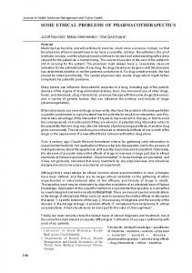
INTRODUCTION Supercavitation provides the potential for an isolated body moving in water to avoid significant viscous losses and reach by that very small cavitational drag as compared to continuos flow. The process of motion of a supercavitating prolate body can be illustrated by the following simple physical model shown in Figure 1. In the case of prolate cavities, the cavitator size is small and the drag is practically independent of cavity form. Thus, the cavity does not depend on cavitator form and is defined solely by the drag. The cavitator pushes motionless fluid aside, and the work of the drag is transformed into kinetic

Fig. 1 Radial flow model

energy, creating practically radial flow at every cross-section passed by the cavitator. Furthermore, the cavitator-induced radial expansion of the cavity section is influenced by the pressure difference between the flow and cavity. Motion of the body in a finite cavity (i.e., in the forward part of sufficiently large cavity) occurs practically without contact with the fluid except for hydrodynamic interaction with a very small forward portion and not large back part of the cavity, provided that the body motion is stable. The lowest drag coefficients, CD , based on cavity midsection, are obtained for slender cavities (assuming that the body is inserted sufficiently close to the cavity walls). The potential for decreasing CD is limited by the maximum aspect ratio of the body, provided adequate strength of the body and 1

adequate external pressure at the place of motion. For highspeed motion in water, values of CD between 0.05 and 0.001 may be reached, and in some cases, drag in a cavity is even comparable to that in air. At super high speeds, realized in water by launching small bodies with mass 0.1-0.5kg, these bodies, through inertia, can reach distances comparable to distances reached in air. Bases of the classical supercavitation theory were developed in considerable part on base ideal incompressible model and this model was of as very good applicable namely for this theory. However here thank to of extreme complex singular structure of solutions application of the modern nonlinear numerical methods had considerable negative experience. In doing so development of the hopeful nonlinear numerical methods had been delayed and hopeful enough numerical solutions were appeared not very ago in spite of considerably more earlier appearance of power enough computers techniques. As the most effective and hopeful for development of classical supercavitation was turned out application of simple heuristic models together with integral conservation laws and (SBT). This way gave the possibility to develop approximate dependencies and methods for calculation of the supercavitation including hopeful prediction of main cavity sizes and form which were verified many times way by experiment. Till recent time the hopeful enough theory of nonlinear numerical prediction of incompressible supercavitation have developed too mainly for steady flows. In doing so the drag calculation can be made by rough enough numerical methods but prediction of the cavity require very perfect and labournes methods. So taking into account very hard negative experience of numerical solutions in the classical supercavitation every apperanse of new numerical methods here first cause alarm from the side of experts in this field and require obligatory hopeful verification of this results. As distinguished with classical theory where all methods and dependencies were verified multiply ways modern situation in the field of super high speed in spite of essential achievements both in the theory and experiments can be defined as dramatic enough. With some assurance we can be sure relay to results on drag and not large ahead parts of the subsonic cavities where theory can be verified by experiment. However unfortunately for super high speeds there are experiments under nature pressure only where cavities are realized of extreme large aspect ratios. This cavities forms liked as needles are not applicable for numerical prediction and verification. Under such conditions the influence of channel walls and free boundary is considerable and methods of this influences account are not developed. The possibilities of serious enough verification are complicated by possible cavitator yield deformation under water entry and abrasive water influence for super high speeds. Under such conditions the most topical from one hand is attempt of the whole situation analysis on base the most hopeful methods had been recommended in the classical theory with making clear main physical effects which is realized in further consideration. From another hand the very important is statement new more perfect experiments which could be hopefully verify the theory. 1. PROBLEM STATEMENT

1.1 Singularities of the theory development for super high speeds. Simples model of cavitation flow Fig. 1 present practically the energy conservation law and in the considerable part is applicable and for super high speeds. However here for M > 1 essential wave loss can be appeared with essential disturbance of the cavitator drag universality from point of view creation of supersonic cavity. Important point is appearance of the classical transonic effects increasing the flow perturbation zone and accordingly inertial properties of the flow. In doing so thank to considerably more as compared to water adiabatic coefficient the water have considerably more wide range of transonic M numbers which is turned out as the most important for applications. From another hand the linearized approach application recognizer identity of the structure of the key integer differential equations on base (SBT) and really definite proximity for the main properties cavitational processes in compressible and in incompressible flows in the water. This proximity give the possibility to apply for the development of the theory of the super high flows key approximation and experience of development of linearized theory in incompressible fluid. With account of proximity of compressibility effects in water and air the base results of the classical aerodynamics here are applicable in the considerable part too. Very important here the results of classical hydrodynamic theory of the explosion in water have been defined fundamental dependencies of unsteady supersonic motion of the water as compressible fluid. The structure of key points of consideration includes follows. On base classical aero-gas dynamics and explosion hydrodynamics presented in the number of known publications and in particular in the [1-6..] the attempt is undertaken to analyze all having theory and experiment dates in the field of the super high speeds from point of view key physical effects understanding with estimation of their possible magnitudes together with development effective enough whole practical approach. One of the key consideration point is application of the known (SBT) by Frankel -Karpovich and Adams Sears [7, 8] on base the theory of the singular perturbations [9] and in particular (MAEM). Started from the most typical steady statement of nonlinear problem for incompressible fluid and it simplification ways the key dependencies and peculiarities of compressible supercavitation flows in the water are presented and analyzed on base of the model of ideal isentropically compressible fluid. On the SBT base the problem is transformed into the problem for integer- differential equations for slender cavities for sub- and supersonic flows, the asymptotic methods of the solution are developed and the problem is analyzed in the acoustic approximation. The (IDE)s with account of walls and free boundary apply to motion of supercavitating bodies in the channel are developed. The linearized theory of unsteady flows is developed. Regularities of the cavitationl drag forming are investigated with account of compressibility and effectiveness criteria are considered. The linearized statement is specified until transonic equation of small perturbed flows and main peculiarities of the transonic supercavitation flows are considered. For final step on base achieved level of understanding the simple effective enough practical approaches 2

are proposed for estimation of supercavitation flows for- sub trans- and not large supersonic speeds of motion. Further some of the most essential problems of the super high speed motion are considered. With account of very fast increasing of the lateral forces for super high speeds even for small trajectory curvature the most appropriate is and is developed the linearized theory of the motion of the supercavitating bodies under inertia along the trajectories of small curvatures. Taking into account essential possible aspect ratios of the bodies the theory is developed with account of hydro-elastics effects; the possibilities of stabilization, resonance effects, dumping and i. e. are considered. 1.2 Nonlinear approach A typical approach is to consider the cavitation problem in the case of steady motion in an unbounded, ideal incompressible fluid, with the Riabushinsky closure (e.g., disc) scheme for the back of the cavity. The cylindrical coordinate system (r, x) shown Fig.1.1 is used. The flow potential ϕ satisfies the Laplace equation. For a given cavitator shape, r = r1 (x) , the impenetrability condition is provided, and for an unknown cavity shape, r = R(x) , the impenetrability condition and the pressure

generalization of the problem statement for unsteady flows. Generalization of the nonlinear statement (1.1-1.5) with account of compressibility is simple enough on base of known equations of aerodynamics barotropically compressible fluid [4-5] using know water state equation [6]. Tait adiabatic curve, expression for sonic speed and Bernoulli on this base are [6] : a) P + B = P∞ + B , n n ρ

b) a = 2

ρ∞

dP n(P + B) = dρ ρ

2 n P + B (U ∞ + u) 2 + v 2 n P∞ + B U ∞ + = + n −1 ρ 2 n − 1 ρ∞ 2

difference, ∆P , between the undisturbed flow and the cavity are assumed. Perturbations at infinity tend to 0: ∂ 2ϕ

1 ∂ϕ ∂ 2ϕ + + =0 , r ∂r ∂r 2 ∂x 2

(1)

(1.1)

2

δ ln1/ δ)

(1)

dr1 ∂ϕ dr1  dR ∂ϕ dR   ∂ϕ  ∂ϕ  ∂r = U∞ dx + ∂x dx   ∂r = U∞ dx + ∂x dx   r =r1 (x) ,   r =R(x) ,

values at infinity for pressure P∞ ; u, v - perturbation of prolong and radial speeds in the flow. For compressibility account in the statement (1.1-1.5) instead of Laplace equation (1.1) the known in aerodynamics system of the equations for speeds potential Φ = Φ (r, x) [4, 5, 7] is applied: 2 2 ∂ 2Φ  1  ∂Φ   ∂ 2Φ  1   ∂Φ   2 ∂Φ ∂Φ ∂ 2Φ 1 ∂Φ 1 1 − + − + =0    −       ∂x 2  a 2  ∂x   ∂r 2  a 2   ∂r   a 2 ∂x ∂r ∂x∂r r r

(1)

(1) r=r1 (x),

(δ2ln1/δ)

(1)

(1)

(δ2ln1/δ)

 1  ∂ϕ 2 1  ∂ϕ 2 ∂ϕ ∆P     +   + U∞  = 2  ∂x  ∂x ρ   2  ∂r   r = R(x) , (ln1/δ)

-1

2

(δ ln1/δ)

(1)

ϕ r,x →∞ → 0 ,

[R = r1 ]x = x0

 dR dr1   dx = dx    x =x 0

1.3)

(1) (1.4)

(1.5)

n   2 ρ∞ U∞ 2  n − 1 2  (n −1)  a) P∗ = c∗ , b) c∗ = 1 1 + − M ∞   2 2  nM∞2   

 n − 1 2  (n −1) c) ρ∗ = 1 + M∞  2  

 n −1 2  d) a∗2 = 1 + M∞  2  

(1.9)

(1.10)

The temperature in the break point is essentially less 100o C . Here by the points × × × the significance of the typical pressure for blow disc again water [12] are indicated too. It is possible with assurance suppose that for water in the range of M ~ 2 − 2.5 and higher and especially for small perturbations flows the model of ideal isentrope compressible flows for cavity boundaries as fixed surfaces is good enough applicable. With account of compressibility the problem is defined by 2 key non dimensional parameters: M ∞ and σ σ = ( P − Pc ) /

Here ρ fluid mass density. For simplicity, the location of separation, x = x0 , is assumed to be fixed, and the system of equations (1.1) must be amended to specify closure conditions. It is appropriate to note that main complexities of the supercavitation flow problem from point of view further linearized approach development is contained namely in the steady statement do not exiting essential difficulties for

(1.8)

Fig 1.2 illustrates closeness of adiabat, dynamical adibat and even in essential part isotherm for water in wide enough range of the pressures (calculations for T = 20o C ) defining the limitation of the problem statement. Intensity of compressibility influence is illustrated by Fig. 1.3 for flow values in the break point pressure, mass density, sonic speed P∗ = P∗104 (kg / cm 2 ) , ρ∗ = ρ∗ρ∞ , a ∗ = a∗a ∞ depend on M ∞ :

1

(1.2)

(1.7)

where: B = 3045kg cm 2 , n = 7,15. Here" ∞ " correspond the flow

2 2 2   n P∞ + B U∞ a2 1  ∂Φ   ∂Φ    = + +  −    n − 1  n − 1 ρ∞ 2  2  ∂x   ∂r    

Fig. 1.1 Schematic of flow

(1.6)

ρ∞ , U ∞2 / 2

M ∞ = U∞ / a ∞

(1.11)

however this parameters are not independent and already depend on each other! Supposed ρ∞ ~ ρo in σ this dependence is:  ρ a2  M = M  1 + σM o2 o o  2B   2 ∞

3

2 o

1− n n

(1.12)

dr12 d2 R2 d2R2 dR2 | − | | 2 x=x1 dx2 dx − dx x=0 + dx x=L = 2σ − ∫ dx 1 |x1 − x| x L-x xo

and illustrated by Fig. 1.4 . Index " o " correspond significance for

P = 1Atm, T = 20o C . 1.3 Acoustic approach on base Slender Body Theory For simplification of the problems accordingly (1.1-1.5) and analogously (1.8, 1.2-1.5) on base of (SBT) Cavitator and cavity as whole are considered as definite slender body with slenderness parameter δ ~ 1 / λ ( λ - aspect ration whole surface). For δ → 0 the equations (1.8) with account of small

− − − − − − − ρ∗

---------- Pθ - Tet adiabat (1.6a)) --- --- --- PD - dynamical adiabat [7]

transformed

(ln1/ δ2 )−1 a)

into

equation

of

acoustics

(1.13)

 S' S' m2 1 L S' (x1) − S' (x)  dx1  ϕ ≈ U∞  lnr + ln − ∫ 4π 4x(L − x) 4π 0 x − x1  2π 

S = S(x) square

of

slender 2

body

lateral

(1.15) sections,

2

m =|1 − M | . Neglected by δ ln1/ δ the system (1.1-2.5) and (1.13, 1.2-1.5) are simplified and on the base (SBT) expansion (1.14, 1.15) are transformed into the problems for integerdifferential equations (IDE)s for slender axisymmetric cavity. In case of slender cavitators this problems are: 2

M 1 d 2 r12 d2R 2 x0 |x=x1 − 2 2 2 2 2 2  2 1 dR d R m R dx 2 dx − ln - 2 ∫ dx   + 1 2  dx  2 2 |x1 − x| 2R  dx 4x  0 (ln1/δ) -1

x

−2

∫

x0

(ln1/δ)-1

(1)

d2R 2 dx 2

|x=x1 − |x 1 − x|

d 2R 2 dx 2

dr12 |x=0 = 2σ dx1 − 2 dx x

(ln1/δ ) -1

[R = r1 (x) ]x =xo ,

(1.14)

x  S'  S' 1 S' (x1 ) − S' (x) m2 ln 2 − dx1  M > 1 ϕ ≈ U ∞  ln r + ∫ 4π 4x 2π 0 x − x1  2π 

2

 dR 2 dr12  b) =   dx  x = x  dx o

Dependence (1.10a)

which can be transformed into Laplace equation by PrandtlGlauert transformation. For M < 1 this is acoustic equation, for M > 1 wave equation. Under each term in particular of the problem (1.1-1.5) the orders of the terms are indicated for δ → 0 , r = δ!r, r! = r / δ = O(1) . Condition at infinity (1.4) are missed and here known (SBT) expansions for flow potential of sourses on the axis are applied [7, 8]:

Here

[R = r1 (x)]x =xo ,

— — — a∗ Dependence (1.10b)

∂2ϕ 1 ∂ϕ ∂2ϕ + + (1-M 2 ) 2 = 0 2 ∂r r ∂r ∂x

M 1 is O(δ) !only. For M > 1 Influence of back closure is essential and here linearized scheme of point closure is applied (1.17b). In dR 2 | at the last term of (1.16) turned out as total dx x=L power of sources for potential ∂ϕ / ∂x (∂ϕ / ∂t) of the closure..

doing so

1.4 Review of selected results First we note some of key results of the incompressible theory. The most effective approach for the first steps uses simple heuristic models, integral conservation laws and perturbation theory. Starting from known research by H. Reichardt, G. Birkhoff and others, the ellipsoidal cavity form and base cavity sizes has been obtained, including the known formula for the maximum cavity radius R k : Rk = Rn

(1.16)

4

cd kσ

(1.20)

where R n is the radius, and c d the drag coefficient of cavitator, ( k ~ 0,94 − 1 ). The essential independence of the expansion of prolate cavity sections was understood. The most clearly this fact since time has been expressed by G. Logvinovich as the known "Principle of independence of the expansion of cavity sections". Investigations by A. Armstrong, D. Gilbarg, M. Plesset, A. May, J.-M Michel, L. Woods, and others should be noted. Effective for number of cases was the application of a plane model describing axisymmetric flow. The asymptotic approach was developed by P. Garabedian, who obtained the known formula for cavity aspect ratio, λ , for small σ : λ2 =

ln1/ σ σ

(1.21)

Also note the known asymptotic of streamlines at infinity ( x → ∞ ) obtained by N. Levinson and M. Gurevich: R 2 = 2 cdo

x 0,5

(ln x )

x  1 ln ln x  1 − 4 ln x + " ~   ln x 0.5

(1.22)

These results represent only a small part of the most important investigations in the field. The creation of known linear theory of plane supercavitation by M. Tulin [10] considerably stimulated development of linearized theory of axisymmetric supercavitation on the basis of known (SBT). This possibility was noted jet in [7]. The methods developed in this theory gave the possibility of considerable advancing further in the field of super high speeds. Hydrodynamics of unsteady water flows with free boundaries as compressible fluid was started in considerable part for explosion hydrodynamics. One of the first here were also penetration into water problems. Note here known researches by A. Sagomonian- V. Poruchikov, V. Kubenko, C. Chou, O. Faltinsen, Yu Yakimiv, A. Terentiev, G. Aleve, V. Eroshin,A. Korobkin, Oshorugin, E. Fontane, V. Gavrilenko and others. One of the first it is need to note the research by G. Aleve on nonlinear numerical prediction of the flows enter into and motion in water axisymmetric bodies with sub- trans- and supersonic speeds [11, 12…] (1980-91), known research by Nishiyama T. and Khan O. [13] (1981) and one of the first experiments for supersonic enter into water for not large supersonic speeds by J. Howard Mc-Millen, E. Newton Harwey, 1946 [14]. There are at present nonlinear numerical calculations for subsupersonic enter into water [15], linearized theory of axisymmetric supercavitation for sub- and supersonic speeds [16-18]. Nonlinear numerical- analytical method for axisymmetric subsonic flows developed in case of finite cavities in [19…]. The attempt of nonlinear numerical calculation for sub- and not large supersonic speeds in case of finite axisymmetric cavities undertaken [20, 21]. The problems of transonic flows have been investigated in [22-25]. Numerical calculations of IDE in the (SBT) approximation have been obtained for subsonic flow [26]. Ones of the first experiments in the field of super high speeds were undertaken in the Institute of Mechanics of MSU [27,28…] (RUSSIA) in the Institute of Hydromechanics of NASU [29,30..] (UKRAINE),in NUWC [31…] (USA). The results on

small scale experiments for super high subsonic speed lunching into water presented in [32] (Russia) in the research of ISL (France) and others. The base model of the supercavitation for super high speeds is model for fixed cavity surfaces what very good is fixed in the all experiments. Recently with account of temperature increasing and vapor creation for hyper high speeds the attempt to predict supercavitation on base mixed models including pure water , two phase mixture and pure vapor waqs undertake n[33]. The problems of supercavtating bodies motion investigated in the known research in the CAHI (Russia), IHM (Ukraine) and other institutes started from 60-70. One of the key problem here is planing supercavitating body and interaction of the stabilizing surfaces with cavity walls. The planing theory is very good developed started from known research by L. Sedov, M. Tulin, A. Terentiev, W. Vorus and others. First solution for planing in the axisymmetric cavity have been obtained by E. Paryshev [34], (1974). Considerable advancing of this problem have been reached in the [35]. Planing theory for super high sub- and supersonic motion in water have been developed by A. Maiboroda [36…] (1999). Linearized theory of motion of supercavtating bodies with account of also hydro elastics effects have been developed in [18, 37] (1980). Approximate equations of motion of supercavitating bodies have obtained in particular in [38, 39] and others. 2. THE LINEARIZED THEORY DEVELOPMENT IN THE SLENDER BODY APPROXIMATION 2.1 Bases of asymptotic approach Linearized theory is based in considerable part on (IDE)s of type (1.16). The bases of asymptoticl approach here had been developed apply to cavitation in incompressible fluid. [41-47] and fully are spread for case of compressible flows. Equations of type (1.6) have principal for δ → 0 differential part. This fact defines 2 key alternatives. From one hand the technology of second order asymptotic solutions (IDE)s on slenderness

Fig 2.1 Asymptotic structure of solutions

parameters is developed. From another hand more rough but more effective for practical things approach on base approximation of (IDE)s by more simple differential equations is developed with application of simple heuristics models and integral conservation laws. One of the alternatives is numerical solutions of (IDE)s [48, 49]. Cavitator and cavity surfaces can be characterized by a single parameter δ , but it actually contains two independent parts Fig.2.1.. In the case of a slender cavity behind a slender cone, we 5

can independently change the cone semi-angle γ and σ → 0 and can consider two independent slenderness parameters for the cavitator - ε (for a cone, ε = tgγ ) and cavity. A solution applicable for any set of parameters would be most preferable, but a general approach has not been developed. However, there are sufficiently well-developed solutions on the basis of single parameters for two typical cases: 1) Regular perturbations case: (2.1) δ / ε = O(1), (σ =O(ε 2 ln1/ ε)), L=O(1)

type (2.1) was formulated. The regular methods of IDE solutions have been developed in [43-45] and first asymptotic solution in case of cone cavitators were obtained. This regular methods is the most simple and further it was applied by a lot authors. However this method thank to essential limitations is small

2) Singular perturbations case

δ ε → 0, (σ 1 on base each of problems (1.16-1.17) and (1.18-1.19) as expansions for cavity form ( for M < 1 also cavity length (2.5)) ( x = 0 in the separation section, slender cavitator length # = 1 ):  2  1 1 ! + ! 2 + ... , L = L + R 2 = δ2 R R + ... 1 o c o 2 2 ln(1/ m 2 δ 2 ) ln(1/ m δ )  

(2.4))

under conditions: ! ! R=R/ δ =O(1) r1 = δr!1 (x), r!1 (x) = r1 (x) / δ = O(1) ; R = δR(x), l = O(1), Lc = O(1) σ(x) = (δ2 ln1/ β2δ2 )σ! (x), σ! (x) = O(1)

(2.5)

and is transformed into sequence of the problems: First order problem M < 1 , M > 1 : σ(x) d 2R o2 = −2 , dx 2 ln1/ m 2δ2  dR o2 dr12  = ,   dx  x =0  dx

6

 R! o2 = !r12  , x =0

(2.6) R o2

x = Lo

(2.7)

M 1 2

0

 dR 1  dR o  d R o  Ro = ln    + −2 dx 2R o2  dx  dx 2  4δ2 (1 + x) 2  −∫1 2

2 1 2

2

2

d 2 R o2 dx 2

0

−2∫

−1

2

2

− x = x1

d 2 R o2 dx 2

| x1 − x |

dx1 −

dr12 dx

2 2 1 2

dr dx

− x = x1

2

σε

| x1 − x |

1 + 1 + σε σε

, Le =

2 1 + σε σε

 l + x 4  2   R12 =ε2 σε  ln x + 1 + σε (lo + x) ln  o −  eσ   lo   δ    L − x  2  zi  ln | zi | 3  2 − ( Lo − x ) ln  o − x  +∑ ai − ln x +  L 2 4 M 1

 L − x   3  zi  ln | zi | 3  2 + ( Lo − x ) ln  o − x   +∑ b i  − x +  L 2 4 0  2 o    

( zi + x )

2

+

2

(2.17)

 z + x     , ln  i  z     i   

bo =4(1 + σε ), b1 = - 4, b2 = − 2σε , b3 = − 2σε

Fig. 2.3 Slender cavity behind slender cone, σ = 0.04 , γ = 10o INCOMPRESSIBLE FLUID:

° °°

——— solution (2.12)

nonlinear numerical calculation

COMPRESSIBLE FLUID:

— — — solution s (2.12): M = 0.6 , - - - - - - dR! 12 dx

M 1 :

= 0, R! 12 x =0

x =0

M = 1.5 .

=0…

(2.10)

Solution in general case as 2 terms of expansion: R2 = r12

xx 2 2  dr2  x x 2σ(x ) d R1 1 1 x− + 1 dx1dx1 + ∫∫ ∫∫ dx2 dx1dx1 2 2 2 2 x=0  dx  β δ β δ ln(1/ ) ln(1/ ) 1 00 00 x=0  

(2.11)

Solution for cone σ = const , M < 1 , M > 1 in quadrates: R 2 = ε2 + 2ε2 x −

σ (ln1/ m2δ2 )

d 2 R12 = ε 2 σε dx 2

M 1 :

σε =

 4  (1 + x ) 1 + σ ε  1 + x   −4 + 2 ln  ln     σε  x    σ δ (lo + x) ( Lo − x ) 

σ 2

2 2

ε ln(1/ m δ )

, σδ =

2 2

δ ln(1/ m δ )

σ and i. e. It is possibly to apply analogously as ln1/ δ2 in SBT δ = 2R m /(l + Lc ) . However this way is not any essential δ = ε , δ2 =

advancing but essentially complicate the solutions so in doing so δ is defined with help step by step method. Fig 2.3 demonstrate solutions results (2.12-2.17) for cone σ = const , δ = ε as compared to nonlinear numerical calculation results for M = 0 A. Terntiev, Yu Kuznetzov, V. Krasnov . 2.3 Forward cavity ( cavities for σ = 0 ) This solutions apply to motion in the forward part of large cavity are not influenced by motion. Interstitial equation and solution Second-order theory with respect to δ requires no fewer than 3 terms of type (1.22) expansions. To obtain the third term, the interstitial equations are extracted from IDEs accordingly (1.16, 1.18). This interstitial equations and its asymptotic solutions for x → ∞ [17, 18] shown for two alternative expansion forms, are ( R n = 1 ): 2

(2.14)

1  dR 2  d 2 R 2 m 2 R 2 1 dR 2 ln =0 −   + 2R 2  dx  dx 2 4 x2 x dx

(

(2.17)

)

2 1 lnln x 1 ln e cdo m 2 x + + ...] ~ a) R = 0.5 [1 − 0.5 4 ln x 2 ln x (ln x ) (ln x )

2 cdo x

2

b)

σ 2

In the solutions obtained the most effective parameters δ are

M 1 : zo = 0, z1 = 1, z 2 = 0, z3 = − Lo ,

(2.15)

( (

) )

2 1 ln 4 m x R = [1 − + ...] ~ 0.5 2 2 2 ln x R (ln x )0.5 ln x 2 R 2    2

2 cdo x

(

)

We also note for M < 1 known energy integral [28]. 7

(2.18)

2

2 1  dR 

2 2

2 2

dR

mR

2

2 dR

= 0,   + 2 ln 2 − 2 x dx 2R  dx  dx 4x

M >1

a)

KSx  9 lnln x 3 lnKSm / 4  x ... ~ + R2 = 1 − 3/2 (ln x)  4 ln x 2 ln x  (lnx)3/2

a)

 3 lnKsm2 /4 Ksx x R2 = 1+ ~ 2 2 3/2 2 ln x /R  (ln x)3/2 ln x2/R2 

(2.19)

(

)

)

 ln4/e2 m2 x  1 x ln s! x ln m2e/ 2   2  − + x2ln x) +  −  x ln e − x ln x  2 ! ! ! ! ! s s s s s     

2

(

 2x  1  2x-1 R2 =ε2  −1 + ln(2x −1) + (x −1)2 ln(x −1) − 2 2   s!  ln1/m ε  2

M1

(2.20)

Cavities behind slender cavitators First-order evenly suitable solutions with respect to the cavitator slenderness parameter, ε , for σ = 0 (inner and interstitial) are obtained based on (1.16-

)

(

)

 3 ln2/m2 + ln2/e x  9 x ln s! x lnm2/2  + − 2 +3 2 − ( x ln 2/e − 3 x ln x)  2 s! s! s! s! s! s!    

}

(2.24)

and accurate enough is defined by first terms of expansions. Solution (2.24) for x → ∞ define K s for cone as: 3/2

3/2  21/3 2   1  2 KS =2εln  2 2 ~2εln 2 2  , K s = 2 cdo ln 2  e m ε   mε  m ε2

Cavities behind nonslender, disc-type cavitators. The inner (near cavitator) solution for a disk-type cavitator is universal and is part of a wide range of solutions for steady and unsteady cavities. This solution zone is essentially non linear. However, it is possible to obtain here for M < 1 a non rigorous, but nevertheless effective, semi-heuristic solution. Supposition that cavity forward part is close to the paraboloid is used. In doing so the interstitial equation (2.17), (given a transformation with respect to x ) is accurate for the pressure distribution on the paraboloid surface. With this approach, the system of approximate equations for a cavity forward part with σ → 0 behind a disc type cavitator and the corresponding approximate solution for R(x) are:

Fig. 2.4 Forward cavities part for σ = 0 I NCOMPRESSIBLE FLUID M = 0 : — — — disc, solution (2.26) on base of (SBT),

——— disc, nonlinear numerical calculation [51], disc, experiment [3], [52] o

— - — - cone γ = 10 solution (2.23) on base of (SBT); COMPRESSIBLE FLUID

M < 1 , M >1 :

disc M = 1 , M = 2 , nonlinear numerical calculation [11, 12] o

− − − − − − − cone γ = 10 M > 1

+

solution (2.22 ) on base of (SBT)

o

+ cone γ = 10 M = 2 nonlinear numerical calculation [11]

+

1.17, 1.18-1.19) and (2.17, 2.19) depend on the cavitator form only through the parameter n ( x = 0 в in the cavitator nose point, cavitator length # = 1 .):  2nx  R 2 = ε2  + (1 − 2n)  , !  s 

M 1



2

3/ 2

 ln( 1/ ε2 )  R = ε 2x     ln( x / ε2 )     2

2

2 cd Rn 2 cdo Rn d R2 2σx − → = , x 2 2 2 dx 2 2 2 (lnx)0.5 ln4 (x+∆) / m R ln4 ( +∆) / m R e R2

R2 = 1 +

(2.21) −

, s! =

ln(x/ ε2 ) ln(1/ ε2 )

 x ~ − 1  (ln x)3.2  x→∞

(2.22)

For cone n = 1 ( ε = tgγ ) this is solutions (2.21,2.22). The solutions for cone as 2 terms of expansion for m = O(1) are :

x=0

= R2n , ∆=0.5Rn  cd + 1/ cd  ,

(2.25)

First order solution (R n = 1) :

ln ( x / ε 2 ) ; ln ( 1 / ε 2 )

x ln x

 2 nx  R =ε + (1 − 2n) 2/3  (s! )    2

s! =

(2.25)

2 (cd − σ) x   4(∆ +x/ e) 2 / β2   ln   [1 + 2 (cd − σ) x / ln(4∆ 2 + x)] 

−

σx 2   4(∆ +x/ e)2 / β2   ln   2 [1 + 2 (cd − σ) x / ln(4∆ + x)] 

(2.26)

Aproach (2.25) is applicapable for estimation in case of not slender cavitators of different form and in case not fixed separation section too. Fig. 2.4 illustrate calculation results cavities for σ = 0 in SBT approximation as compared to nonlinear numerical prediction and experimental date. Calculation results shown not essential influence compressibility on forward parts of the cavities M < 1 which is essentially 8

increase for increasing of M towards transonic range. However for M >1 compressibility influence can be considerable: forward parts of cavities for M >1 especially for not slender enough cavitators can be considerably more narrow thank to essential wave loss as compared to M = 0 , M < 1 . 2.4 Slender cavity behind small cavitators The solutions here are the most important for practical use where we have long enough cavities behind of disc type cavitators. The outer solution describe the largest part of the cavity, which is sufficient for estimation of form, dimensions, volume, etc.. Neglecting cavitator size O(δ 2 ln1/ δ 2 ) and assuming the cavity semi-length Lk = 1 as given (actually found during matching) the problem for equation (1.16) for M = 0 , M < 1 is: 2

An asymptotically equivalent dependence for Lk was obtained by variation method [54], thus confirming theory for M < 1 . By similar way on base equations (2.19) and solutions (2.20), (2.30) the dependencies of R k , L k for M > 1 are found too:    0.5 + ln 2  Lk = R n 1 −  3/ 2 1   1  2 ln 2δ  ln 2 2   m 2δ2   m δ  Ks

R k = R n δLk ,

1 σ=δ2 / ln 2 2 m eδ

(2.33)

(2.34)

Structure of evenly suitable solutions. Through matching, a first-

βR 1 dR  d R − ln  + 2 2 2 R  dx  dx 4(1+ x)(1− x) d2R2 d2R2 dR2 dR2 | | | − +1 x=x 2 1 dx2 dx − dx x= −1 + dx x=+1 = 2σ(x) − ∫ dx 1 |x1 − x| 1+ x 1− x -1 2

2

2

2

2

 R 2 (x) = 0  ,  R 2 (x) = 0  x= − 1  x= + 1

(2.27)

We solve for the general case σ = σ(x) as an expansion: R 2 = δ2  R 2o + R 2−1(ln1/ β2δ2 )−1 + ...  

(2.28) Fig. 2.6 Slowly changing parameters

For σ = const , a second-order solution applicable for different δ (but σ / δ 2 ln1/ δ 2 → 1 ) is: R2 =

INCOMPRESSIBLE FLUID:

▬▬▬▬ dependence for µ (2.41dd),

——— dependence for k (2.42e);

 (1 − x2) + x2 ln4 − ln(1 + x)(1+x) − ln(1 − x)(1−x)  2 (1 x ) − +   ln1/ δ2  ln1/ m2δ2 

a)

σ

2 2

1/ m δ σ= 2 ln e λ 1

→ δ=1/λ

b)

λ σ= 2 ln e λ 2

(2.30)

=

R 2n

cd σ

 ln 2 / e  1 + 2  ln1/ m2δ2   2 2

Lk = R n

cd ln1/ m δ  ln e / 2  1 − ln1/ m2δ2  σ  

COMPRESSIBLE FLUID:

M = 1.7 .

order evenly suitable solution (interstitial and outer, R n = 1 ) is obtained [25, 27]: M = 0 , M 1 is solved by fully similar way on base likely transformed problem for supersonic IDE and conserve for M > 1 form of dependence (2.29b): 2 2 σ  (1− x2) + x2 ln4+ln(1+ x)(x −x−2) −ln(1−x)(x−x )  R2 = (1−x2) +  ln1/δ2  ln1/ m2δ2  

nonlinear numerical calculation [51]:

=

Ks (ln x)

3/ 2

x−

σ x2 → ln1/ σ x →∞

M >1 :

x ln x

3/ 2     ln( 1/ ε2)  x  − σ (x −1)2 R = ε 2x − 1 →    ln( x/ ε2)    ln1/ σ (lnx)3.2     x→∞ 2

9

2 

(2.37)

(2.38) (2.39)

Expressions (2.36-2.39) are of qualitative nature only and describe specific structures of the solutions. Practical dependencies for prediction of cavity sizes For practical use there here for M = 0 number of approximate dependencies thoroughly and multiply [3] and also on base nonlinear numerical calculations [51]. The most convenient here is direct dependencies on σ . Asymptotic approximations on base (2.31, 2.31) applicable in wide enough range of M < 1 start from λ ~ 3 − 5 including super slender cavities of R k , Lk , λ for σ = const behind of type disc cavitators are: a) R k = R n

cd kσ

,

b) Lk = R n

cd 2µ / k

(2.40)

σ

here κ n , κc define accordingly wave loss on cavitator and cavity. Dependencies (2.44) give very strong increasing of wave loss on cavity when cavity become considerable more slender as compared to cavitators. Here however it is need to note that expression of type (2.31) even for M < 1 is essentially depend on appropriate slenderness parameters use. Jet more complicated can be situation for M >1 where thank to very wide in water transonic range the zone of applicability the solutions on base acoustic approach can be considerably shifted in the range of M essentially more high as compared to 1. Numerical calculation [21] also detects fast enough increasing of k (1/κ) for increasing of M after M ~ 1 . So for present time dependence (2.44с) can be considered as of qualitative nature only and require obligatory verification by experiments. Fig. 2.5, 2.6 presents calculations results λ (σ) и µ(σ) , k(σ) for m = 0 as compared to nonlinear numerical calculations for steady cavity behind disk with symmetric scheme of Riabushinsky closure. 2.5 Unsteady flows Similar to (1.16- 1.17) problem for unsteady flow in the coordinate system connected with motionless fluid are [40]: 2

1  ∂R 2  ∂ 2 R 2 m∗2 R 2 −  + 2 ln 2  2R  ∂t  4[ x n (t) − x ][ x c (t) − x ] ∂t ∂ 2 r12 ∂ 2R 2 ∂ 2R 2 ∂ 2R 2 − − 2 2 2 x (t) e ∂t x = x ∂t ∂t x = x ∂t 2 1 1 dx1 − ∫ dx1 − − ∫ x1 − x x1 − x x n (t) xs (t)

Fig. 2.5 Dependence λ = λ (σ)

xs (t)

INCOMPRESSIBLE FLUID:

——— (2.41c), — — — (2.29b),

∂R 2 ∂r12 dx (t) ∂t x =xe (t) dx n (t) ∂t x =xn (t) 4∆P(x,t) − e + = ρ dt xe (t) − x dt xn (t) − x

nonlinear numerical calculation [51]. COMPRESSIBLE FLUID: •

dependence (2.41c) for M = 0.7 ; - - - - - - - dependence (2.41c) for M = 1.7 . •

•

1 1.5 1 1.5 c) λ = ln 2 : → d) µ = ln 2 , 2 mσ σ mσ

(2.41)

 ln 2 / e  e) kβ = 1/ 1 + 2  ln 5/ m2σ  

(2.42)

2

With account of solutions structure in case of slender cavitators expression for maximal cavity radius more appropriate to present as:  κc  R 2m = R 2n 1 + do  σ  

For

(2.43)

aspect ratio dependence is conserved as (2.41) for M < 1 . However for R m defining for M < 1 situation is considerably more complicated. At present it was possible to find dependence for " κ " in case of slender cavitators only. In doing so dependence (2.43)and κB for cone are: M >1

κ c   a) R 2m = R 2n 1 + B do  , κ B = κ n κc , σ  

c)

 2 e κc =  ln 2 2  m ε

  2eλ 2  /  ln 2 m  

2

b) κn = 1 −

 ln(1/ m 2 ε 2     ~    ln(λ 2 / m 2 )    

 ∂R 2 ∂r12  = ,  R 2 = r12  , R 2 (x, t) = 0     t =ts (x)   x =xe (t) ∂t   ∂t t =ts (x)

ln(1/ m 2 ε 2 )

2

(2.44)

(2.46)

Here t is the time, and x n (t), [xs (t), t=t s (x)], x e (t) are laws of motion for the cavitator nose, separation section , and cavity end, respectively. Equation(2.45) with account weak enough influence of M can be applied at least for M < 1 for some typical in the process significance of M ∗ (m2 = m∗2 ) . The problem (2.45-2.46) also have to be added by initial conditions. The solutions of the (2.45-2.46) for cavity form is given as expansions f likely as in steady case:   1 1 R 2 = δ2 R! o2 + R! 12 + ... , L c = L o + + ... 2 ln(1/ δ 2 ) ln(1/ δ )  

(2.47)

and is transformed into the sequence of the problems. First order problem: ∂ 2 R o2 ∂t 2

1

(2.45)

=

4∆P(x, t) ρ ln(1/ δ2 )

 ∂R2 ∂r2  , Ro2 = r12  ;  o= 1  t =ts (x) ∂t   ∂t t =ts (x)

Second order problem:

10

(2.48a)

2

m∗2Ro2 1  ∂R o2  ∂2R12 ∂2R o2 −  − 2 + 2 ln 2 2 2R 0  ∂t  ∂t ∂t δ 4[xn (t) − x][xe (t) − x]

∂Ro2 ∂r12 ∂t x=x (t) dx (t) ∂t x =x (t) eo n =0 + n xe (t) − x dt xn (t) − x

xo

+∫ 0

 ∂R12  , R12 = 0 , R 2 (x, t) = 0 = 0 .  t =ts (x)  o  x=xeo (t)  ∂t  t =t (x)  s

(2.48b)

Here for δ it is possible to use δ = ε, δ 2 ln(1/ δ 2 ) = σ∗ and i.e. where σ∗ - is typical for the process cavitation number. Without of any prevalence here likely as in SBT it is possible to use typical aspect ratio of cavitator and cavity as whole too. The solutions of the problem (2.48-2.49) is not difficult and detailed is described in [45]. Here in the most part cases second order analytical solutions are possible. However from one hand alike solution are not essential value for applications thank to limitations of type (2.1). From another hand it give such long expressions which give not any possibility to analyze physics of the results, so here the most appropriate is using this solutions in the quadrature form likely as (2.11). More correct statement of the problem is possible on base IDE with lag argument of type ( on base sources with lag time distribution on the axis):

L 2 2 1 1 1 d2r12 1  dR − −  dx1 + | dx + |   1 ∫ 2 x=x1 2 x=x1  dx Hf Hf  xo dx Hf Hw 

1  ∂R 2  ∂2R 2 R2 + − ln   ∂t 2 4[xn (t) − x][xc (t) − x] 2R2  ∂t  ∂2r12 ∂ 2R 2 ∂ 2R 2 ∂ 2R 2 xe (t) (x1,t∗) − (x1,t∗) − 2 2 2 ∂t dx − ∂t ∂t 2 dx − − ∫ ∂t 1 1 ∫ x1 − x x1 − x xn (t) xs (t)

  1 1   1 1 − −   =  2 2 2 H H w   (x − x) + m h (x1 − x) 2 + m 2 h 2W  f 1 f 

4∆P(x,t) , ρ

t∗ = (t −

| x1 − x | ) a∞

(2.49)

Here a ∞ - sonic speed.. The solution of the problem for this IDE fully similar as (2.47-2.48). Note here that the most effective for applications methods for prediction of unsteady flows were developed on base differential equations approach and they will be presented in further consideration. 2.7 Walls and free boundary influence This solutions are very important for understanding of experiments results. The superposition approach for estimation of influence of wall and free boundary on cavity behind slender cavitator is used. Flows for M < 1 One wall + one free boundary, h w , h f - distance from cavity axis accordingly up to wall and free boundary:

   

(2.51)

Small distances case h w , h f → 0 wall free boundary case: 2

2

xo

h 1 d R  d R m R ln w2 −   + 2 R2  dx  d x2 hf 4(x-xo )(L - x) ∫0 2

2

2

2

2

d2r12 |x=x 1 dx2 dx1 − |x1 − x|

dr12 d2R2 d2 R2 dR2 | − |x=0 |x=L x=x 2 2 1 dx dx − dx − ∫ dx + dx =2σ 1 |x1 − x| x L-x xo L

(2.52)

Free boundary only: 2

1  d R2  d2 R 2 R2 ln 2 = 2σ  + 2  2 2 R  dx  dx hf

(2.53)

Wall only:

xs (t)

∂R2 ∂r12 (x1,t∗) (x1,t∗) ∂ ∂ t t x1 =xe (t) dxn (t) x1 =xn (t) dx (t) = − e + xn (t) − x dt xe (t) − x dt

(2.50)

dr 2  1 dR2  1 1  1  +  1  −  +  −  = 2σ  dx  Hf Hw x=0  dx  Hf Hf x=L

2

=

d2r12 |x=x 1 dx2 dx1 − |x1 − x|

1  d R  d2 R2 m2 R2 − ln  + 2  2 4(x-xo )(L - x) ∫0 2 R  dx  dx dr12 d2R2 d2R2 dR2 − | |x=0 | L 2 x=x1 2 dx dx − dx dx x=L − ∫ dx + 1 |x1 − x| x L-x xo

∂ 2R 2o ∂2r12 ∂2Ro2 ∂2Ro2 − − 2 2 2 xs (t) ∂t xe (t) ∂t ∂t ∂t 2 x=x1 x=x1 dx1 − ∫ dx1 − − ∫ x1 − x x1 − x xn (t) xs (t) dx (t) − eo dt

xo

2 2

2

2

xo

h m hwR 1 d R  d R ln w2 −   + 4 R2  dx  d x2 hf 4(x-xo )(L - x) ∫0 2

2

2

2

d2r12 |x=x 1 dx2 dx1 − |x1 − x|

dr12 d2 R2 d2 R2 dR2 | − 2 |x=0 | 2 x=x1 dx dx − dx dx x=L = σ − ∫ dx + 1 |x1 − x| x L-x xo L

(2.54)

Flows for M > 1 Wall + free boundary:

d2r12 | 2 x=x1 1 dR  d R m R dx − ln 2∫ dx1 −   + |x1 − x| 2 R2  dx  d x2 4(x-xo )2 0 dr12 d2R2 d2R2 − 2 | |x=0 x 2 x=x1 dx dx dx −2 ∫ dx1 − 2 |x1 − x| x xo 2 2

xo

+2 ∫ 0

2

2

2

xo

x 2 2 1 1 1 d2r12 1  dR − | dx +  1 ∫ 2 |x=x1  −  dx1 + 2 x=x1  dx Hf Hf  xo dx Hf Hw 

dr 2  1 1  +  1  −  = 2σ    dx  Hf Hw x=0

11

2

(2.50)

  1 1   1 1 − −   =  2 2 2 H H w (x1 − x)2 - m 2 h 2W  f   (x1 − x) - m h f

   

(2.51)

Small distance case h w , h f → 0 Wall + free boundary: d2r12 xo 2 |x=x 2 2 2 2 2 2 2 1 h   1 dR d R m R ln w2 dx1 − − 2 ∫ dx  + 2  2 2 |x1 − x| 2 R  dx  dx hf 4(x-xo ) 0 dr12 d2R2 d2 R2 | − 2 | 2 x=x1 dx dx − 2 dx x=0 =2σ −2 ∫ dx 1 |x1 − x| x xo

(2.52)

x

2

1  d R2  d2 R 2 R2 ln 2 = 2σ  + 2  2 2 R  dx  dx hf

(2.53)

Wall only: d2r12 |x=x 1 hw m hwR 1 d R  d R dx2 + ln 2 dx1 − −   ∫ 2 2 2 dx 4(x-x )(L x) |x x| − 4R  dx hf  o 1 0 2

2

2

2

xo

2

dr12 d2 R2 d2 R2 − | | 2 x=x1 dx2 dx − 2 dx x=0 = σ − 2 ∫ dx 1 |x1 − x| x xo

(2.54)

Asymptotic solution method here are fully alike as (2.4-2.10, 2.11-2.15, 2.16). Wall influence is alike as parallel moving supercavitating body influence and till definite limit increase inertia property of the flow and increases influence of transonic effects. Influence of free boundary decreases inertia properties of the flow and can fully neutralize transonic effects influence. 3. CAVITATIONAL DRAG 3.1 Cavitator drag Cavitators drag in water includin hydrodynamic and hydrostatic component can be presented by known dependence: 2 ρU∞ , cd = cdo + ∆cdh + cdp , b) cd = cdo (1 + σ) 2

(3.1)

However for not slender of type disc cavitator hydrostatic pressure and cavity influence ∆cdh on drag are small. Known dependence for disc for M = 0 is (3.1b) where, for a disk, cdo ~ 0.82 − 0.83 . As numerical calculations show [12] the drag of type disc cavitators in wide enough range M < 1 , M > 1 can be not bad estimated on dependence for pressure in break point. and here for preliminary estimation it is possible to apply dependence of type: M 1 : cd = 0.82c∗ + σ

n   2  n − 1 2  (n −1)  1 1 + M − ∞   2  nM∞2   

× × × × on Fig. 1.3. The drag of slender cavitatoirs depend on similar effects more essentially and her number result were obtained in the research [54-58 ] and others. For M < 1 general enough dependence for drag for unsteady flow by speed U n are:

a) D = Sn cdo (1 + σ)

L

a) D = cdπR2n

-------- dependence (3.5): 1 - γ = 5o , 2 - γ = 10o , 3 - γ = 15o

× × × - nonlinear calculation [51]

Free boundary only:

2

Fig. 3.1 Dependence cd = cd ( γ, σ) for M = 0

(3.2)

b) cdo = 2ε2 ln

( m∗x

= (4 / 3)ρR 3n

for a disk) [3]. Hydrodynamic mass pressures for blow against water on base date [12] indicated by

χn , mε



c) m∗x = 2ε2  ln 

χn  πε2 #3 ρ 3 mε 

(3.3)

Here ∆Ps is pressure difference in the separation section # , Sn ,length and square of cavitator in the separation section, L = ( Lc + l ) / # , L c ~ L o - cavity length defined by dependence of type (2.15). cdo , m∗x cavitator drag coefficient for steady flow and cavitator added mass σ = 0 ,; χ n - defined by cavitator form and in particular for cone is: χn =

 2  2 / 1 −  e  5 ln(1/ m 2 ε 2 ) 

(3.4)

Value of µ is defined by dependence of type (2.41) and in particular as µ = 0.5 ln(1/ m∗ σ∗ ) with using typical for the unsteady process values. For steady flow dependence (3.3a) is: D = Sn

2   ρU ∞ σ  2 cdo (1 + σ) −  ln L +  + σ   2  2µ  3 

(3.5)

and combine both known dependencies: a) cd ~ cdo (1 + σ)

b) cd ~ cdo + σ

(3.6)

Fig. 3.1 illustrate calculation results on dependence (3.5) as compared to date of nonlinear numerical calculations [51] For M > 1 there are absence of back influence of the flow : (3.7) cd = cdo + σ and for slender cavitator the draq for M > 1 is defined by its form only. In particular for cone on base of known dependence [7] we have:

The unsteady drag component can be estimated on blow added m∗x

dU ρU2n  ∆P   2 + m∗x n − Sn  s  ln L +  − ∆Ps  2 dt 2 3 µ    

cd = cdo + σ = 2ε2 ln

3.2 Cavitational drag 12

2 1 +σ e mε

(3.8)

Drag coefficients CD and CDf ( CD o ) are some characteristics of the supercavitation motion effectiveness. CD is drag coefficient relative to the cavity midsection. CDf for motion in the forward cavity part express drag coefficient of the forward cavity part respect to section with radius R b at x = L$ λ $ = R b / L$ . For σ ~ 0 , CDf = C Do Second-order dependencies for like disc cavitators for σ → 0 ( δ ε → 0 ): M 1 1, 2, 3 - nonlinear calculation [11,12] M = 0.3, M = 1, M = 2 ,

5 - dependence (2.25) -

Fig. 3.2 - CDf for forward part of the cavity -------- CDo - dependence (3.5) — - — - CD

4 - dependence (3.8)

dependencies for finite cavity on base ellipsoidal cavity form only applicable both for M < 1 , M > 1 with account of correspond dependencies for " κ ". For M < 1: κ=κb = 1/ k, For M > 1: κ=κB = κ n κc :

- calculation for λ f significance at middle section,

———

-----

CD - calculation for significance of λ f = λ , CDf - estimation of by dependence (3.6)

2

accordingly for σ = 0, σ = 0.01, σ = 0.02, λ f = λ / 2 .

a)

Similar dependencies for M > 1 δ ε → 0 , σ = 0 in case of slender cone are: 2

4

(3.8) For σ = const here it had more appropriate to apply dependence for slender cavitator of type (2.44) Cdo =

cdo 1 + ( κ n κc ) / σ

(3.9)

Fig. 3.3 illustrate compressibility influence on forward part of the cavities ( σ = 0 ) on base dependencies (3.5, 3.8) recalculated

1 3  3  ln(1/ σ)  CV =  π   2 4   κ  (λ ) 4 / 3 2

b)

2

 ln(4λo2 / m2  1 ln2λo / m  ln(2λo )2 / m2  M > 1 : CDo = ln   ~   2 2 2 4λo em λo  ln(2/ m2ε2  8 ( 2λo )2  ln((2/ ε)2 / m2 )  1

γ = 10o M ~ 1.4

2

3 4/3 1 3 3   σ CV =  π  4   κ3/ 2 ln(1/ σ) 

(3.12)

Analysis of the results shows: - 1)movement in the finite cavity is more effective the more slender the cavity is, with the main limitation being the practically attainable aspect ratio for a real body; 2) movement in the forward part of the cavity results in considerably less cavitational drag, and the action of pressure can decrease supercavitation effectiveness; 3) for M > 1 , a significant decrease in effectiveness appears due to wave losses. For slender cavitators, this effect increases as the slenderness decreases; 4) Numerical calculation confirm appearance of 13

essential wave loss on cavity which are of the most large value for like disc cavitators. 4. Transonic flows Due to considerably different adiabatic coefficients in water and air, water has a very wide transonic range where flow is gradually transformed from pure subsonic to mainly supersonic flow as M gradually increases. In the case of disc cavitators for M ~ 0.95 − 0.97 and σ ~ 0.03 − 0.02 in the cavity region, a supersonic zone of finite size appears from the moment when the

× [1 +

ln(4 / e2 ) ]]} 2 2 ln(1/ ε (1 − )) 5ln(1/ ε 2 )

(4.3)

Averaging for another slender cavitators is alike. Fig. 4.1 illustrate very good coinciding of calculation results for cdo on base dependencies (4.2, 4.3) for cone γ = 10o as compared to nonlinear numerical calculation [11]. Analogously the attempt to estimate aspect ratio is undertaken. It is Here it is need to note that thank to that M ∞ and σ are not

independent and M ∞ = M ∞ (σ) - dependence for aspect ratio of type (2.29, 2.41c) it is need to precise with account of (1.12) : 1−n

2 n  2 ρo ao  σ +σ M M ln(1.5/ | 1   -1|) o 2B  ln(1.5/ σ | M∞2 −1|  2 λ = = σ σ Applied as typical average value of M on the cavity: 2 o

Fig.4.1 Transonic drag of slender cavitators

γ = 10o × × × nonlinear numerical calculation [11] σ = 0 1, 2 - acoustic dependencies (3.5) M.< 1 , (3.8) M. > 1 σ = 0

cone

3 - calculation by dependencies (4.2, 4.3)

cavity is the surface of critical speeds. For M = 1 , this zone becomes infinite and at the forward and back regions of the cavity shock waves start to appear. Thus, two finite zones of subsonic speeds bounded by critical surfaces behind these shock waves are created. The flow for M ~ 1 is characterized by considerable increase of the lateral dimensions of the perturbation zone. Account of second order terms for expansion of (1.8) give the possibility to obtain transonic equation in water applicable also the range of M ~ 1 similar to known Karman Gudetrley equation: ∂ 2ϕ ∂r 2

+

m∗2c =| M ∞2 [1 + (n + 1)σ] − 1 |

)

(4.1) Below likely as in transonic aerodynamics [8] the attempting is undertaken to approximate transonic equation by acoustic equation. With account of considerable shift of subsonic flow near slender cavitator into supersonic Mach range transonic term for M. > 1 in (4.1) is averaged and as typical value of M used typical value of M on the slender cavitator surface. In doing so with account of that main part of the flow near cavitator is subsonic - cavitator drag for M. > 1 is estimated on base dependency for M.< 1 . It is supposed also that Mach range where essential effects of the mixed zone of sub- and supersonic flows existence is not large. Typical m in particular for cone estimated by (4.3)and drag coefficient estimated as: cdo = ε 2 ln(

4 2 / ε 2 (1 − )) em∗n 5ln(1/ ε 2 )

m∗n = 1 − M ∞2 {1 − [(1 + n)ε 2 [ln(1/ ε 2 (1 −

2 5ln(1/ ε 2 )

(4.2) ))] ×

(4.5)

cavity aspect ration for M. > 1 and not large zone for M. > 1 can be estimated by dependence:

( n + 1) M∞2 ∂ϕ  ∂ 2ϕ = 0 1 ∂ϕ  +  1 − M∞2 −  r ∂r  U∞ ∂x  ∂x 2

(

(4.4)

Fig.4.2 Cavity aspect ratio in transonic flow 1, 2 - calculations on acoustic dependence (4.4) 3 - dependencies (4.4-4.6) with account of (4.4). Points i i i nonlinear numerical calculation [21]

(4.6) ln(1.5 / σm∗2c σ Fig. 4.2 demonstrate estimation of transonic cavity aspect ratio results on base dependence (4.4 4.6) as compared to attempt of nonlinear numerical calculation [21]. For practical use here can be applied curves 1 and 3 up to its crossing. Calculations are for λ2 =

σ = 0.0268 , values of M ∞ are recalculated for this σ . Date of [21] approximately recalculated for constant σ = 0.0268 on base weak changed value of λ 2 σ . 5. PRACTICAL APPROACHES 5.1 Differential equation for the slender axisymmetric cavity in steady flow IDEs of type (1.16, 1.18, 2.45 ) and also (2.49) respectively have a principally differential part for δ → 0 . Main idea is the possibility of approximation of the IDE in the outer field by a 14

simpler differential equation and apply initial conditions with help of integral conservation law instead of matching. The system of equations for defining a slender axisymmetric cavity behind a small cavitator in steady flow is [42,43, 59]: µ R2

x =0

= 0,

d 2R 2 dx 2

2

dR dx

+

∆P(x) 2 ρU ∞ /2

= 2 x =0

b) R k = R n

cd kσ

,

D 2 kπµρU ∞

. (5.1)

∂t 2

t = t n (x)

+2

= 0,

∆P(x, t) =0, ρ ∂R 2 ∂t

cd 2µ / k σ

(5.2)

Here the expressions for R k , Lk ,λ are the same as defined by dependencies of type (2.40 - 2.44), µ has clear physical sense as the inertial coefficient for cavity sections expansion. Equation (5.1) can be presented as the energy equation Values of µ and k are found through best approximations on the basis of secondorder equations and solutions and usually in such a way that it would be possible to more precisely define maximum cavity radius and length for specific case studies. The system (5.1) describe the most part (outer solution) of the cavity excepted small nonlinear zone near cavitator (of type disc) which can be added after the solution. Key point for using of this equations with account of compressibility is to know 2 key values. This is value µ which can be found both for M < 1, M > 1 and with account of (4.4-4.6) can be estimated also for transonic range including M ~1 . Second key values are: for M < 1 κβ = 1/ k ~ (0.95 − 1) defined by dependencies of type (2.42). But sitution for M > 1 including very wide for water transonic range is more complicated. Here it need to find the value of type κB (2.44) . But for rough estimation it is possible to hope that increasing of values κB after M ~1 . will not be very fast at lest till small supersonic Mach Numbers: M ~1.1-1.2 and it is possible to neglect by this effect and suppose that κB ~ 1 . Not very fast increasing of the κB is defined numerical prediction [21].

also

by the

5.2 Unsteady slender axisymmetric cavities. An important characteristic of steady solutions is that µ and k are sufficiently weak functions of aspect ratio both for M < 1, M > 1 including transonic range. For M < 1 this fact is demonstrated by Fig. 2.6 for base cavity sizes. However instead of perfect independence we have a very weak dependence of the sections expansion on aspect ratio and specific flow conditions. Taking account of the weak dependence for µ , k , analogous to (5.1), unsteady equations for a slender axisymmetric cavity for variable pressure in the coordinate system connected with the stationary fluid are:

D(x) kπµρ

=2 t = t n (x)

(5.4)

Here the cavitator drag D(x) is a quasi-steady dependence at the moment of passing through the motionless fluid at section x . In the most important range λ ~ 5 − 20 , the constant µ ~ 2 in case of M = 0 . is frequently used. For compressible flows this values can be precise with help some typical significance of m∗ for the unsteady process. More precisely µ = µ(x) can be defined as

2cd σ 2 ⋅x − x kµ 2µ

c) Lk = R n

R2

∂ 2R 2

=0 ,

Solution (5.1) for σ = const defines a known ellipsoidal cavity form (5.2a) and dependence for R k (4.2b): a) R2 = Rn

µ

(

)

µ ≈ 0.5 ln 1.5 / m∗2 σ based

on the

quasi-steady

dependence of σ w when passing through the section, x . The transonic influence can be account of to on base (4.4-4.6) Equations (5.4) even on the basis of steady dependencies for µ are applicable for estimation of cavities which can be considerably different than ordinary steady ones and even yield realistic qualitative results for step changes in cavitator speed and, hence, drag. This has been verified many times and it's accuracy is within 5 - 7 %. A small zone near the disk, is added for the final calculation step. 5.3 Effective calculation method for the steady and unsteady cavity for M < 1 Many problems in supercavitation are essentially nonlinear, and hence nonlinear numerical calculations are particularly important. Taking into account the small gap between the cavity and the body is key for accurate calculation of the cavity on the basis of the ideal incompressible model in the case of a disc cavitator and Riabyshinsky closure scheme. It is important that the solution have a complicated nonlinear structure, and when solving a concrete numerical calcullation problem, it is necessary also to provide acceptable accuracy. This is extremely important for essentially multi-variants unsteady flows. Using the system of equations (5.4) provides the potential to estimate cavity form and sizes but not for adequate description of the whole cavity. Thus, the idea of effectively approximating an IDE by an ordinary differential equation is applicable for the entire solution region, including the zone near cavitator of disc type. Specific flow singularities are accounted for based on an expansion of the outer equation and based on this method, the significance of the integral part of IDE can be estimated. Analogously (2.25), the system of equations (5.4) is refined for disc-type cavitators and transformed into a system of the equations for the prediction of unsteady cavities: ∂ ∂R 2  1 2∆P(x, t) =0,  µ(x, t) + ∂t  ∂t  ρ µ(x, t)

a) b)

∂R2 ∂t

=2 t =tn (x)

D(x) , R2 = R2n , c) R 2 = R e2 , t = t e (x) t =tn (x) k(x)ρµn 2

2

1 4 ( xn +∆n ) − x x − ( xe +∆e ) d) µ(x,t)= ln  2 2 m∗2R2 [xn − xe + (∆n +∆e ]

15

1−  

0.4[xn − x][x − xe ]  , [xn − xe ]2 

e)

µ n = ln

2∆ n , m∗ R n

g) ∆ n =

Rn  1   cd + .  2  cd 

(5.5)

The solution is determined based on the problem for a simple ODE (5.5a) containing dependencies (5.5d - 5.5g) and additional conditions of type (5.5c) for finding cavity length. For cavities not significantly different from ordinary steady ones: ∆ e ~ ∆ n , the radius of back closure R e ~ R n , and the correction k is applied based on the steady solution. A more precise value of ∆ e is defined based on (5.5g) where R e is defined based on (5.4) and here it is possible to make quantitative assessments . Analogously (5.1, 5.4) it is possible to hope that the system give the real possibility to estimate cavity form in the whole range of M till not large M ~ 1.1-1.2 . In doing so any small not axisymmetric cavity deformation for whole enough M range can be predicted with help known theory [60].

oscillates, and bends, and, as a result, the local speeds and angles of attack of it different components that interact with the cavity are significantly different. The cavitator in this system marks the curved trajectory of the centers of expanding cavity sections. In doing so, the cavitator imparts to the sections a definite lateral speed and inertial impulse and after that, the sections and body components interact with finite time lag. Besides, a cavity for motion can be deformed under different external factors, some of the most significant being lateral gravity influence and gas injection, and even for motion of a rigid body in an empty cavity connected with the possibility of appearance of power oscillation processes. Thus, we have a complicated complex process including rigid and hydro elastic body oscillations under the action of cavity deformations and waves on its surface which can appear for steady and unsteady motion. Hydrodynamic with cavity interaction effects A key problem is planing on the cavity surface and essential to this problem is the

Fig. 5.1 Cavity behind disc in incompressible fluid ———— system of equations on base SBT (5.1),

Fig. 5.1 demonstrates the accuracy of the solution based on the system of equations (5.1) for a steady cavity behind a disc cavitator for σ = 0.04 , M = 0 as compared to a nonlinear numerical calculation [51]. 6. SUPERCAVITATING BODY MOTION 6.1 Some peculiarities of the motion The most convenient approach is the application of the equality conditions of inner forces and moments projected to normal and tangential axes of the trajectory of motion y = y(x) . In the case of level motion, the system of equations for the trajectory are: MU s

dθ dy − Fn + Mg cos θ = 0, = tan θ , dt dx 2

J

d (θ + α) dt 2

+ M =0.

nonlinear numerical calculation [51].

application of the strip model for the hydrodynamic interaction with the cavity. In most cases, the linear presentation of the angle of attack is used. The possibility of a sufficiently effective presentation of lateral forces based on the added mass, m , at separation. Given a sufficiently wetted back part of the body, known linear theory for slender body lift [4, 8] is applicable. But for some cases, for example in the case of the angle of attack for a disk-type cavitator, this dependence can be nonlinear. It is important to account for compressibility for planing for at sub-, trans-, supersonic speeds [36]. Hydro elastic effect account A model problem based on differential equations for an elastic beam [61] is: a)

(6.1)

Here M is the body mass, J is the longitudinal moment of inertia, t is the time, Us (t) is the velocity component along the trajectory defined by the addition to equation (6.1), α, θ are the angle of attack and the angle tangential to the trajectory, respectively. Equations (6.1) are written in with Fn as the normal component of the main vector, and M as the main moment of all inner forces acting on the body, including hydrodynamics forces. In general, the process of motion can be imagined as follows. A moving cavitator creates a cavity surface and after that, the body moves on the surface. The trajectory of the cavitator and the trajectory of all parts or the body interacting by hydrodynamic way with the cavity (planing, stabilization, etc.) do not coincide with the trajectory of the center of mass. The body rotates,

b) c)

∂2  ∂2y  ∂2y =0 2  Ei(x) 2  + M (x) ∂x  ∂x  ∂t 2  ∂3 y 2 ∂y  ,  Ei(x) 3 − mUs  ∂x ∂x  x =−a  ∂2y , ∂x 2 x =−a

∂2y . ∂x 2 x =a 1

∂3y , ∂x 3 x =a 1

(6.2)

Here, i(x) = i∗ i (x) is the linear moment of inertia M (x)

and

= M∗ M (x) is the mass of beam sections. E is the elastic

modulus. The center of mass is located at the coordinate, x = 0 . Distances a and a 1 are measured from the center of mass to the back and front of the beam, respectively. In the model statement, the lift force, for simplicity, is situated at the body back section. m is the separation added mass at the back body section. A linearized solution of the problem (6.2) is determined using a 16

quasi-rigid approximation for

( M∗ / Ei∗ ) → 0

. Equation (6.2a) is

twice differentiated with respect to x and second order terms are neglected. Using integral conditions of conservation, all forces and moments on the beam, (6.2) is solved for M = const and is transformed to the simple equation1 a)

J kα =

b)

d 2η + k α amUs2η = 0 , dt 2

1 , 1 + mUs2 / K b

c)

K b = ξb

Ei m . a2

(6.3)

essential influence of real lift force position shift to forward this date can give to high estimation and can be as preliminary oriented only. 6.2 Linearized equations of motion One basic model is for nearly straight, inertial motion at nearly constant speed, where the problems of vertical and lateral motion can be considered essentially separately. Prolong motion. The elementary model of motion is applied to very high speed launching in water, with inertial motion and drag based on the quadratic law of velocity, so that only cavitator drag is considered. The maximum distance, X* , traveled by inertia along the cavitational trajectory is defined by the expression: 1/3

 G  X∗ = 0.23   ρbg 

1/3

ρb 2/3  0.71  (κ)  ln  ρ  σo 

4

/ σo 3 ,

3

σ∗ = σoe 4 .

b)

(6.4)

where G is body weight, ρb is mass density, g is gravity, and σo , σ* correspond to the initial and final moments. It is

supposed that at the final moment, surfaces of the body and cavity coincide ( κ -characterizes how much of the cavity if filled by the body at the final moment.) Maximal distance is reached, based on the relationship of (6.4b) for σ∗ , given optimal body aspect ratios. Note here too the investigations by T. Gieseke Lateral motion The linearized model applies to very high speed launching, with subsequent near straight body motion by inertia. The body has a wetted stabilizing part at the back, and the hydro-elastic effects are accounted for based on generalization of 1

The equation (963) obtained (1997) together with Yu. Scosarenko.

d 2 ∆y d ∆y m + khm + k h ∆y = 0 , dx 2 dx J d ∆y , = − J (αo − Jωo ) , dx x =− Jω

a)

b)

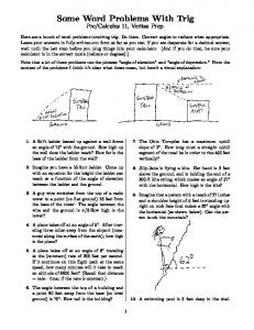
Here, J is the longitudinal moment of inertia of the beam, i m is the value of i(x) at the center of mass, and the value of η ≈ α (i.e., close to the angle of attack of the body at the center of mass). The solution for M = const have been defined significance of ξ b ~4,8 for this case. Physically hydro elastic effects are manifested here by more small attack angles in the back base of body as compared to it's values for the rigid body. Fig. 6.1 illustrates the results of hydro elastic effects action on attack angle at the back body section in case of model case of supercavitation flow of metallic body for E ~ 4 × 1011 n / m 2 of near paraboloid form with wetted back part of body. The estimation date for k α = k α ( M ) on base formulas (6.3) depend on Mach Number are presented for three body aspect ratios λ b ~ 5, 10, 15 and rough estimation of ξ b ~11.5. With account of

a)

the model problem (6.2, 6.3). Neglecting small lateral forces on the disk-type cavitator and accounting for sufficiently slow damping of velocity, the system equation for the trajectory y = y(x), y = y / a, x=x/a is given as:

c)

∆y x = 0

o

∆y = y − J (α o − Jωo ) − (θo + Jωo )x ,

d) k h = 1/[1 +

mUs2 Ei ] , 1 = [ 1 + 1 ] , K b∆ = ξb∆ 2m , (6.5) a Kh Kh K s K b∆

Here, α o , θo , U o , ωo , are the initial angle of attack, the angle tangential to the trajectory of the center of mass, , linear velocity, and angular velocity, respectively. a is the distance between centers of mass and pressure. m is the separation-added mass of the back wetted part of the body, combined with any stabilizers interacting with cavity surfaces, M, J are the mass of the body

-------

Fig. 6.1 Hydro-elastic effects k α (6..3) for body aspect ratios λ b ~ 5, 10, 15

and the longitudinal moment of inertia. E, i m are the modulus of elasticity and lateral moment of inertia at the section of the center of mass, K b∆ is the body rigidity ( K b - without influence of lift shift), defined in a special way, K s is the stabilizer rigidity. The problem (6.5) defines lateral trajectory coordinates relative to the axis inclined with respect to the direction of initial motion and by using the classical equation of harmonic oscillations with damping, can be solved separately for α, θ,(α + θ). Physically, this fact corresponds to lateral and angular oscillations of an elastic body, where energy is transformed from one type of oscillation into another, with energy then transformed into lateral energy in the wake behind the body. Even this simple linearized model for the case of a rigid body uncovers the most important properties of supercavitation motion connected with the manifestation of intensive oscillations, with definition of key parameters of this process. It is important that this model is significantly unsteady and not quasi-steady. This model provides the possibility to account for and investigate a number of additional significant effects including cavitator action. On base this models were predicted the resonance frequencies for lunching into and motion in the water not large supercavitating bodies for speed near 1000-1500m/s. In doing so this frequencies turned out close to the own elastic frequencies of the bodies and more close when more high speed. It was discovered 17

that hydro elastic effects and elastic stabilizers can very strongly decrease this frequencies. This effect turned out as more effective for more elastic steel bodies as compared to for example tungsten bodies. From another hand steel bodies have less effective damping characteristics. Main prevalence of the system of type (6.5) is simplicity which give possibility by very simple way estimate possible resonance zones, influence of different stabilizers on damping processes and trajectory deflection, i. e.. CONCLUSIONS Simple heuristic models, together with integral conservation laws, SBT models based on MAEM and nonlinear numerical calculation methods provide the most effective approaches for development of the supercavitation applications for high speed motion in water. At present, based on the investigations of many authors, a sufficiently complete theory has been developed, with possibilities for calculating steady and unsteady supercavitation motion for most practical cases. The least developed theory in for the case of super high trans-. and supersonic speeds in water. The most topical at present is the development of sufficiently promising prediction methods for cavity size and form for M > 1 including transonic range and in particular ways of hopeful prediction of maximal radiuses of the cavities in this range, in particular for the transonic range, and especially experimental verification of the theory at this range of speeds. REFERENCES 1. Birkhoff G., Zarantonello E., 1957, " Jets, wakes and cavities." - New York: Academic Press. - 406 p. 2. Gurevich M. I., 1978, "The theory of jets of ideal fluid." Moscow: Nauka. - 536p. 3. Logvinovich G. V. , 1969, "Hydrodynamics of flow with free boundaries" - Kiev: Naukova Dumka. - 216p. 4. Liepman H. W., Roshko A., 1957, "Elements of Gasdynamics" New York -London: John Willey Sons Inc., Chapman Hall Ltd .- 518p. 5. Cherny G. G., 1988, "Gasdynamics." Moscow: Nauka.- 424p. 6. Yakovlev Yu. S., 1961, "Explosion hydrodynamics".Leningrad: Sudostroenie. - 312p. 7. Francl F. I. Karpovich E. A., 1948, "Slender bodies Gasdynamics." - Moscow: GosTechIzdat. - 175p. 8. Ashley H., Landahl M., 1969, "Aerodynamics of Wings and Bodies", Mashinostroenie, Moscow, 318p. 9. Van Dyke M., 1964, "Perturbation Methods in Fluid Dynamics." - New Yourk - London: Academic Press. - 310p. 10. Tulin M. P., 1964, "Supercavitating flows - small perturbation theory " J. Ship Res., 7, 3, pp.16 - 37. 11. Aleve G. A., 1983, "Separating flow of circle cone by transonic flow of water," J. Trans. of AS USSR, MFG, 1, pp. 152-154. 12. Aleve G., 1988, "3-D problem of disc entering in compressible fluid". Trans. AN USSR, MFG, 1,pp. 17-20. 13. Nishiyama T. and Khan O., 1981, "Compressibility effects upon cavitation in high-speed liquid flow (Transonic and supersonic liquid flows) //"Bulletin of the Japanese Society of Mechanical Engineers 24, 190.

14. Howard Mc-Millen J. , Newton Harwey E, 1946, "A Spark Shadow graphic Study of Body Waves in Water" , J. Applied Physics, Vol. 17, 7, pp. 541-555. 15. Terentiev A. G., Chechnev A. V., 1983, "Submersion of plate and disc of finite mass into compressible fluid" J. Trans AN USSR, MFG, 3, pp.147-179. 16. Serebryakov V.V., 1992, Asymptotoc solutions of axisymmetric problem for sub- and supersonic separate flows in water under zero Cavitation Number", J. DAN of Ukraine, 9, pp.66-71. 17. Serebryakov V.V., 1994, "Asymptotic sollutions of the developed cavitation flows problems in the slender body approximation", Kiev, J. Hydromechanics, 68, pp.62-74. ( The paper for 7th USSR symposium on theoretical and applied mechanics, Moscow 1991). 18.Serebryakov V.V., 2002 "Models of the Supercavitation Prediction for High-Speed Motion in Water"// Proceedings of International scientific school "High speed Hydrodynamics, 2002, Jun. 16-23, Chebocsary, Russia, pp.71-92 (Invited lecture) 19. Zigangareva L. M. , Kiselev O. M., 1998, "Subsonic cavitational flow by compressible fluid for small Cavitation Numbers", Trans RAN, 4, pp. 27-34 20. Vasin A. D., 1996, "Calculation of axisymmetric cavities behind disk in subsonic flow of compressible fluid", J. 21. Vasin A. D., 1997, "Calculation axisymmetric cavities behind disk in supersonic flow", J. Trans RAN, MFG, 4, pp. 5462 22. Adam S., Schnerr G.H., 1997 " Instabilities and bifurcation of non-equilibrium two-phase flows."// J. Fluid Mechanics Vol. 348, pp 1-28 23. Schnerr G.H., 1993, " Transonic aerodynamics including strong effects from heat addition."// Computer and Fluids, Vol. 22, No. 2/3 pp 103-116 24. Schnerr G.H., 1995" Multiphase flows: Condensation and Cavitation Problems "// Proc. 6th ISCFD - International Symposium on Computational Fluid Dynamics, September 4-8, 1995, Lake Tahoe, USA (eds. Hafez, M., Oshima, K.). John Wiley, pp. 614-650 25. Schnerr G.H., 2003" Unsteady nonadiabatic transonic twophase flows."// Proc. IUTAM Symposium Transsonicum IV, September 2-6, 2002, Göttingen, Germany (ed. Sobieczky, H.). Kluwer Academic Publisher 26. Vargnese A., Uhlman J., Kirschner I., 1997, Axisymmetric slender-body analysis of supercavitation high-speed bodies in subsonic flow , Proc. of conference in Rhode Island , pp. 185200. 27. Eroshin V. A., Romanenko I. I, Serebryakov I. V. Yakimov Yu. L., 1980, " Hydrodynamic forces under strike of the blunted bodies against surfaces of compressible fluid", J. DAN AS USSR, MFG, 6, pp.44-51. 28. Yakimov Yu L., 1987, " Flows limit of water", in the book "Mechanics and technical progress, MFG, vol. 2." Moscow: Nauka, pp. 7-25. 29. Savchenko Yu. N., Semenenko V. N.., Serebryakov V. V., 1993, "The experimental investigation of supercavitation in subsonic flow"//J. DAN of Ukraine, 2 , pp 64 - 68. 18

30. Vlasenko Yu., 2002, "Experimental investigationsof supercavitation flows at subsonic and transonic velocities", Proceedings of International scientific school "High speed Hydrodynamics, 2002, Jun. 16-23, Chebocsary, Russia, pp197204 31. Kirschner I., 1998 "Supercavitating Projectile Experiments at Supersonic Speeds"//High Speed Body Motion in Water, Agard-R-827, France, pp.35(1-4). 32. Bivin Yu., Gluchov Yu, Permiakov Yu., 1985, " Vertical enter rigid bodies into water"// Trans. of AS of USSR, MFG, No6, pp.3-7. 33. Saurel R. Cocchi J.P., Butler P.B. , 1999, "Numerical study of cavitation in the wake of hypervelocity underwater projectile"// J. Propulsion and Power.,15, 4, pp. 513-523. 34. Paryshev E.V., 2002 "The plane problem of immersion of an expanding cylinder through cylindrical free surface of variable radius"// Proceedings of International scientific school "High speed Hydrodynamics, Jun. 16-23, Chebocsary, Russia, pp. 277284. 35. Kring D., Fine. N., Uhlman J., Kirschner I., 2000, "Unsteady cavitational model, using 3-D method of boundary elements", J. Applied Hydromechanics, 2(74), 3, pp. 53-59. 36. Mayboroda A. N., 2002, " Planing for sub- and supersonic speeds"// Proceedings of International scientific school "High speed Hydrodynamics", 2002, Jun. 16-23, Chebocsary, Russia, pp..271-276 37. Serebryakov V. V., 1996 "Investigation of sub- and supersonic body motion in water by inertia", Nikolaev, Ukraine, Proc. of second scientific school " Impulse process in continuum medium mechanics", pp.50-51. 38. Putilin S. I., 1998, "Stability of Supercavitating Slender Body during Water Entry and Underwater Motion", France: Agard-R-827, pp. 27.1-27.14. 39. Rand R., Pratar R., Ramani D., Cipola J., Kirschner I., 1997, " Impact dynamics of a supercavitating underwater projectile"// Proc. of conference in Rhode Island, pp 175-183. 40. Serebryakov V.V., 1978, "On statement of linearized problems of axisymmetrical supercavitation in unsteady flows", in the paper set "Mathematical methods of hydrodynamics flows investigations." - Kiev, Naukova Dumka, pp. 58-62. 41. Serebryakov V.V., 1973, "Asymptotic solution of the problem on slender axisymmetric cavity", DAN of Ukranian SSR, ser. A , 12, pp.1119 - 1122. 42. Serebryakov V.V., 1974, "Ring model for calcullation of axisymmetric flows with developed cavitation," Kiev, J. Hydromechanics, 27, pp.25-29. 43. Logvinovich G. , Serebryakov V., 1975, "On methods of calculation of of slender axisymmetric cavities shape", Kiev, J. Hydromechanics, 32, pp. 47-54.

44. Serebryakov V.V., 1976, " Asymptotic solutrion on slender cavity form behind slender body"// Kiev, J. Hydromechanics, 34, pp. 48-52. 45. Serebryakov V. V., 1990, "Asymptotic solutions axisymmetric problems of the cavtational flow for slender body approximation," The papers set "Hydrodynamics of high speeds", Chebocsary, Russia, Chuv. SU, pp. 99-111. 46 Serebryakov V.V., 1986 "Dependencies to limit of unsteady flow of slender axisymmetric bodies"// Kiev, J. Bionics, 20, pp. 21-32. 47. Serebryakov V.V., 1998 Asymptotic approach for problems of axisymmetric supercavitation based on the slender body approximation // Proc. of 3 International symposium on cavitation, Grenoble, , 1998, vol. 2 pp. 61-70. 48. Nakatani H., Nakatani G., Mijai I. A finite cavity flow about a slender body of revolution in a tube // Bull. JSME. 1979. -22, N170. 1092-1098. 49. Vorus W., 1986, "Ambient supercavitaties of slender bodies of revolution" 3, N3, J. .Ship Res., 215-219. 50. Grigorian S. S., 1959, "The approximate solution on separate flow of axisymmetric body", J. PMM, 23, 5, pp. 951-953. 51. Guzevsky L. G., 1979, "Numerical analysis of cavitation flows." - Novosibirsk, Russia, Preprint N40-79 of CO AS USSR, Heat-Physics Institute. -36p. 52. Brennen C., 1969, "A numerical solution of axisymmetric cavity flows", J. Fluid Mech, 37, 4, pp. 671-688. 53. Petrov A. G., 1986, "Asymptotic expansions for slender axisymmetric cavities"// J. ПМТФ, 5, pp. 45-49. 54. Plesset M.S., Shaffer P. A. 1948, Drag in cavitating flow //Reviews of modern physics. Vol. 20, N1. 228-231. 55. Sagomonian A. Ya., Poruchikov V. B., 1970, "3-D problems of unsteady motion of compressible fluid." -Moscow: MSU.120p. 56. Taic O. G., 1975, "Prolong flow of axisymmetric body with free boundary", Russia, J. PMM, 39, 1, pp.185-188. 57. Nesteruk I. G., 1982, "Some problems of axisymmetric cavitational flows"// J. Trans of AS USSR, MFG, 1, pp. 28-34. 58 Serebryakov V. V., 1989, "On equations limit of the slender axisymmetric cavities theory for unsteady flow", 23, pp. 18-33. 59 Serebryakov V., 1981, "Calculation of slender axisymmetric cavity forms in unsteady flow for a number of characteristic cases" Kiev, J. Hydromechanics, 44, pp. 86-94. 60. Shoravlev Yu., 1973, "Methods of perturbations theory in 3D stream flows", CAGI Proceeding 1532. - 23p. 61. Bisplinghoff R. L., Ashley H., Halfman R. L., 1956, "Aeroelastcity."- Cambridge: Adisson-Wesley Publ., 800p.

19