parallelograms (Fig. 2.1 and Fig. 2.2). Figure 2.1. Figure 2.2. Solution: Let O be an arbitrary finite point in the plane of the quadrangle ABCD. The reflection Φ has.
Anale. Seria Informatică. Vol. XI fasc. 1 – 2013
79
Annals. Computer Science Series. 11th Tome 1st Fasc. – 2013
SOME PROPERTIES OF REFLECTION OF QUADRANGLE ABOUT POINT* Boyan Zlatanov Plovdiv University “Paisii Hilendarski”, Faculty of Mathematics and Informatics * The research is partially supported by NI13 FMI-002 ABSTRACT: We show the power of the simultaneous usage of GeoGebra and Maple for generalizing and proving of geometry problems. We present a simple school problem, where with the help of the dynamics in GeoGebra new geometric properties are recognize and then we prove them with the help of Maple. We state an open problem for an investigation. We suggest a new construction for GeoGebra that can optimize the construction process in the extended Euclidian plane. KEYWORDS: Dynamic Geometry Software, Computer Algebra Systems, reflection about point, conic section, loci, homogenous coordinates.
1. INTRODUCTION Dynamic Geometry Software (DGS) and Computer Algebra Systems (CAS) have been widely used in teaching mathematics, solving problems and research. A classical usage of DGS is presented in [Pec12], where the problem is visualized and the dynamics is used to recognize geometry properties like invariant points, lines, circles etc., then using this knowledge a conjecture is stated and proved or disproved. Some applications of GeoGebra for the finding of loci are made in [Ant10, GE11, Pet10, Sor10]. We would like to mention that in many cases DGS helps students not only to visualize the problem or to suggest new geometric properties, but also helps to hint ideas for the proof [FT10, KTZ13]. A good example for generalizing and discovering of new types of objects is given in [Bar11], where a new class of central cyclides is found and a full classification of them is made. Another benefit of the DGS and especially of GeoGebra is that they give a linking of Geometry and Algebra as it is shown [HJ07]. We would like to mention that DGS could help the teacher to optimize the teaching process [Cho10, KTZ13]. The project Fibonacci [***] has made a large step towards introducing of GeoGebra to the Bulgarian teachers. There are geometric problems that are possible to be solved without to much writing, once we have observed the idea of the proof [KTZ13], but there are problems in geometry, when the solution involves analytic geometry, that requires a lot of writing and calculations [GN08, GN11]. The CAS are of great help for these type of problems as it is shown in [Ger09], where Maple is used for calculating of non
trivial geometric problems. A classical geometric problem that involves a minimization is investigated in [Ger09], where Maple is used for the actual calculations of the examples, and DGS is used for the visualization of the problem. Hilbert geometry in a triangle is investigated in [MRG10]. The illustrations of some of the concepts such as Hilbert distance, projective and affine coordinates are presented with Maple. The problem of determining the minimum surface area of solids obtained when the graph of a differentiable function is revolved about horizontal lines is investigated in [Tod08]. Solutions for this problem are given with the help of Maple and several potential difficulties are identified, when using CAS. A Maple procedures based on integration and transformation methods is presented and used to evaluate signed areas and volumes. The procedures are designed with formal parameters which can be easily used or modified by instructors and students [XYS12], which shows another benefit of the CAS – the possibility to generate procedures that can be used for large classes of problems. It is shown that CAS enables to solve many elementary and nonelementary problems of classical geometry, which in the past could not be solved for the complexity of involved equations or the degree of the problem [Kar98]. Following the above ideas we present a simple school problem and with GeoGebra, we recognize new geometric properties and we prove them with the help of Maple. The Maple file and the sketches can be downloaded from http://fmi-plovdiv.org/GetResource?id=1440. 2. PRELIMINARY RESULTS We will start with a classical school problem, which can be solved with basic facts from the Elementary Geometry. Problem 1: Let ABCD be a quadrangle and the points P and P′, Q and Q′, R and R′ be the midpoints of the segments AB and CD, BC and AD, AC and BD, respectively. Prove that the quadrangles PQP′Q′, PRP′R′ and QRQ′R′ are parallelograms (Fig. 1).
Anale. Seria Informatică. Vol. XI fasc. 1 – 2013
80
Annals. Computer Science Series. 11th Tome 1st Fasc. – 2013
The solution uses the well known properties of the mid segment of a triangle (PQ // AC // P′Q′ , PQ′ // BD // P′ Q ). The generalization of the above problem as like as the generalization of the main problem require the quadrangle ABCD to be considered as a complete quadrangle in the terms of the projective geometry: Definition 1:([Cox49], p. 14) Four points A, B, C, D, of which no three are collinear, are the vertices of a complete quadrangle ABCD, of which the six sides are the lines AB, AC, AD, BC, BD, CD. The intersections of opposite sides, namely, U = AB ∩ CD, U = BC ∩ AD, W = AC ∩ BD are called diagonal points and are the vertices of the diagonal triangle .
Figure 1.
The present investigation is made in the Euclidian plane extended with all its infinite points and its infinite line. Therefore we will use homogeneous coordinates. Let us remember: If (x,y) is a point in the Euclidean plane we will put as its homogenous coordinates in the extended Euclidian plane (tx,ty,t), t∈R\{0}. For any t1,t2≠0 the points (t1x,t1y,t1) and (t2x, t2y, t2) are one and the same finite point. The points at infinity are denoted with (x,y,0). For any t1,t2≠0, x2+y2≠0, the points (t1 x t1 y,0) and (t2 x,t2 y,0) are one and the same infinite point. Note that the triad (0,0,0) is omitted and does not represent any point. The origin is represented by (0,0,1). The equation of a line in Cartesian coordinates is l:ax+by+c=0 and in homogenous coordinates is l:ax+by+ct=0. The equation of a line l, passing through two points (a1,b1,t1) and (a2,b2,t2) is: x l : a1
y b1
t t1 = 0 .
a2
b2
t2
The equation of a curve of the second power in Cartesian coordinates is k:ax2 + by2 + 2cxy + 2dx + 2ey + f=0 and its equation in homogenous coordinates is k:ax2+by2+2cxy+2dxt+2eyt+ft2=0. For a quadratic form k : ax 2 + by 2 + ft 2 + 2cxy + 2dxt + 2eyt = 0 the matrixes
a c A=c b d e
d e , f
a c A33 = c b
are used for determining the type of the curve k. It is degenerated if and only if det(A)=0. The curve k is: parabola if and only if det(A33)=0, hyperbola if and only if det(A33)>0, ellipse if and only if det(A33)