Figure 5: The farfield amplitudes in the forward direction, F(Ëz,t)=Ëx · F(Ëz,t), for the two spheres given ... every closed surface Sr â V around the point r. The medium in a volume V ..... John Wiley & Sons, New York, second edition, 1975. [4] O. D. ...
CODEN:LUTEDX/(TEAT-7112)/1-15/(2002)
Some results extracted from the time domain version of the optical theorem
Anders Karlsson
Department of Electroscience Electromagnetic Theory Lund Institute of Technology Sweden
Anders Karlsson Department of Electroscience Electromagnetic Theory Lund Institute of Technology P.O. Box 118 SE-221 00 Lund Sweden
Editor: Gerhard Kristensson c Anders Karlsson, Lund, December 15, 2002 �
1 Abstract The time domain version of the optical theorem is discussed. The theorem is derived from the optical theorem in the frequency domain by the Parseval’s relation. It expresses the sum of the scattered and absorbed energies in terms of the scattered farfield in the forward direction. From the theorem, causality, and reciprocity a number of results concerning the scattered and absorbed energies from a plane pulse that is scattered from bounded objects are obtained. Some of these results are verified by numerical calculations.
1
Introduction
Consider a plane wave pulse with a length of half a nanosecond that is scattered from the three perfectly conducting objects in figure 1. It is a very hard numerical problem to obtain the scattered field with good accuracy since the geometry of the objects are complicated and since the multiple scattering effects cannot be neglected. Nevertheless, the scattered energy can be obtained within ten minutes on a 300 MHz PC or Mac, with a simple numerical program based on Mie scattering. The key to this numerical simplification is the optical theorem in the time domain. From that theorem one can prove that the scattered energy for the case in figure 1 is three times the energy that is scattered from one perfectly conducting sphere of radius one meter. The optical theorem in the frequency domain is well studied, cf [7]. The theorem relates the total scattering cross section to the scattering amplitude in the forward direction. Less attention has been paid to the time domain version of the optical theorem, cf [2] and [5]. It relates the sum of the scattered and absorbed energies to the farfield amplitude in the forward direction. The paper [5] presented results that can be extracted from the time domain optical theorem. In the current paper some of these results are reviewed and some new results concerning reciprocity and polarization are presented. Also, new concepts such as the domain of dependence of a scattering object, equivalent and independent scattering objects, and independent pulses are introduced. The incident plane wave propagates in the positive z−direction. The corresponding electric field is given by E i (z, t) = E 0 (t − z/c0 ),
(1.1)
where the vector E i (z, t) lies in the xy-plane since the wave is transverse. It is assumed that the incident pulse has finite length, which implies that E 0 (t) is zero outside some time interval t0 < t < t1 . The leading edge of the pulse then arrives at z = 0 when t = t0 and the trailing edge when t = t1 . It is possible to have t1 = ∞ if E 0 (t) goes to zero when t → ∞.
2
2m z
Figure 1: Scattering of a plane incident pulse with length t1 − t0 < (π/3 − √ 3/2)/c0 ≈ 0.6 ns from three perfectly conducting objects. The two lower objects have cavities shaped like circular cones. The optical theorem implies that the three objects are equivalent and independent for the incident pulse. The scattered energy is then equal to 3Wsphere , where Wsphere is the scattered energy for the uppermost sphere with the other two objects not present.
2
The scattered field
The scattered field from an incident plane pulse can be expressed in terms of the induced charge and current densities in the scattering region by the Jefimenko’s equation, cf [4]. Thus � � � � � ˙ (r � , tr ) ρ(r , t ) , t ) 1 ρ(r ˙ J r r E s (r, t) = rˆ u + (2.1) rˆ u − 2 dv � , 4πε0 V |r − r � |2 c0 |r − r � | c0 |r − r � | where rˆ u = (r − r � )/|r − r � |, tr = t −
|r − r � | c0
(2.2)
is the retarded time, and where the dot denotes time derivative. The far zone is defined as the region where the scattered field can be approximated by E s (r, t) =
F (ˆ r , t − r/c0 ) , r
(2.3)
where F is the farfield amplitude and r = |r|. The continuity equation implies that 1 ρ(r, ˙ tr ) = −∇� · J (r � , tr ) + ∇� tr · J˙ (r � , tr ) = −∇� · J (r � , tr ) + rˆ u · J˙ (r � , tr ) (2.4) c0
3
1.4 m
εr = 1
2m εr = 16
εr = 16
Figure 2: Two spheres that are equivalent for an incident pulse of length less than 6 ns. The permittivity in the shaded regions is εr = 16 and everywhere else there is vacuum. where ∇� = (d/dx� , d/dy � , d/dz � ). From Jefimenko’s equation, the continuity equation, and Gauss law it is seen that � � � µ0 F (ˆ r , t − r/c0 ) = − (2.5) J˙ (r � , tr ) − rˆ J˙ (r � , tr ) · rˆ dv � . 4π V When the scattered farfield amplitude is integrated in time one obtains �∞ F (ˆ r , t − r/c0 )dt = 0,
(2.6)
−∞
where it has been assumed that there are no currents in the object before, and after a long time after, the pulse impinges. Thus the following general result holds for the farfield amplitude: The time mean value of the farfield amplitude is zero, in all spatial directions, regardless of the time-dependence of the incident plane wave. This result is utilized in the definition of independent incident pulses below.
3
The optical theorem
The optical theorem can be derived in the frequency domain, cf [7], [1], and [3], and in the time domain, cf [2] and [5]. It is also possible to use the Parseval’s relation to transform the theorem from the time domain to the frequency domain, and vice versa. In this section the frequency domain theorem is presented and the time domain version is derived from it by the Parseval’s relation.
4
3.1
The optical theorem in the frequency domain
˜ (ˆ Let E˜0 (ω) and F r , ω) be the Fourier transforms of the incident field and the farfield, respectively. Thus � ∞ ˜ E 0 (ω) = E 0 (t)eiωt dt −∞ � ∞ (3.1) iωt ˜ (ˆ F r , ω) = F (ˆ r , t)e dt. −∞
The sum of the scattered power, Ps , and the absorbed power, Pa , is given by 1 P (ω) = Ps (ω) + Pa (ω) = Re {s(ω)} 2
(3.2)
where s(ω) is the sum of the scattered and absorbed complex powers. The frequency domain optical theorem implies that s(ω) = −
4π ˜ ∗ ˜ (ˆ iE 0 (ω) · F z , ω), kη0
(3.3)
where k is the wavenumber, η0 is the wave impedance in vacuum, and where the asterisk denotes complex conjugate. Thus it is sufficient to know the farfield amplitude in the forward direction to obtain the sum of the scattered and absorbed powers.
3.2
The optical theorem in the time domain
In the time domain the scattered energy is given by 1 Ws = η0
�∞ � �
|F (ˆ r , t� )|2 dΩdt�
(3.4)
−∞
where dΩ = sin θdθdφ and where the surface integration is over the unit sphere. The absorbed energy is given by �∞ � � Wa = − −∞
� ˆ (E(r, t� ) × H(r, t� )) · ndSdt
(3.5)
S
ˆ where the surface S is a closed surface that circumscribes the scattering objects, n is the outward directed unit normal vector to that surface, and E, H are the total electric and magnetic fields. Let f (t) and g(t) be two square integrable functions with Fourier transforms ˜ f (ω) and g˜(ω). The Parseval’s relation then reads � ∞ � ∞ 1 ∗ f˜(ω)˜ g ∗ (ω)dω, f (t)g (t)dt = (3.6) 2π −∞ −∞
5 Since s(ω) is the spectrum of the sum of the scattered and the absorbed powers, it is seen that the sum of the scattered energy, Ws , and absorbed energy, Wa , is given by � ∞ � ∞ 1 2 ˜ (ˆ ˜ ∗ (ω) · i F W = W s + Wa = s(ω)dω = − z , ω)dω. (3.7) E 2π −∞ µ0 −∞ 0 ω The Parseval’s relation is applicable and gives � t� � 4π t1 � W = Ws + W a = − E 0 (t ) · F (ˆ z , t�� )dt�� dt� . µ0 t0 t0
(3.8)
This is the time domain version of the optical theorem. Many of the results presented in this paper are derived from the following observation: The sum of the scattered and absorbed energies is uniquely determined by the farfield amplitude in the forward direction during the time interval [t0 , t1 ].
4
Implications
There are a number of fundamental results that can be derived from the time domain version of the optical theorem. Some of these were presented in [5] and they are here complemented by new results
4.1
Scattering from several objects
Consider a case where an incident plane pulse of length t1 − t0 is scattered from a region with N objects. The objects are defined as energy independent for that incident pulse if N � W = Wi , (4.1) i=1
where Wi is the sum of the scattered and absorbed energies for object i with the other objects not present. This is the case if the multiply scattered waves are delayed at least a time t1 − t0 relative the wavefront of the incident field. An example of scattering from independent objects is depicted in figure 1. In that case the total scattered energy is the sum of the three energies for each of the three objects with the other two not present.
4.2
Domain of dependence and equivalent objects
The part of a scattering object that for a given pulse can contribute to the sum of the scattered and absorbed energies defines the domain of dependence for the energy for that pulse. For a non-dispersive scattering object the domain is given by all points for which the shortest travel time for any ray that passes through that point is delayed less than the length of the incident pulse, i.e. less than t1 − t0 , compared to the wave front of the incident field. Two objects that have identical domain of dependence are
6
10
Ws (pNm)
8 6 4 2 0
0
5 time (ns)
10
Figure 3: The integral in Eq. (5.1) as a function of the time tc for the spheres in figure 2. The incident wave is given in figure 4. equivalent in the sense that they have the same sum of the scattered and absorbed energies. As an example the three perfectly conducting objects √ in figure 1 are equivalent for an incident pulse with pulse length t1 − t0 < (π/3 − 3/2)/c0 ≈ 0.6 ns.
5
Geometry and incident wave
A plane wave impinges on a bounded region where one or more scattering objects are situated, cf figure 1. Outside the scattering region it is assumed to be vacuum. Figure 2 shows two objects that are equivalent for the incident pulse in figure 4. The permittivity in the shaded regions is εr = 16, and everywhere else there is vacuum. The equivalence is checked numerically in figure 3 where the integral 4π − µ0
�
tc
t0
�
E 0 (t ) ·
�
t�
F (ˆ z , t�� )dt�� dt�
(5.1)
t0
is given as function of tc for each of the two objects when the incident pulse given in figure 4 impinges. When tc > t1 ≈ 8 ns the values of the integrals are seen to be constant. According to Eq. (3.8) the values of the integrals are then equal to the scattered energy. The farfield amplitude for the two objects is given in figure 5. It is seen that the farfield amplitudes for the two objects deviate after the incident pulse has passed but the scattered energies are the same.
7
E i (t) (V/m)
0.5
0
−0.5
5 time (ns)
0
10
Figure 4: The function E0 (t) = (T − t)/t0 exp(−(t − T )2 /t20 ), where T = 5 ns and t0 = 1 ns, as a function of t. The corresponding incident wave E i (z, t) = ˆ E0 (t − z/c0 ) is used for the figures 3 and 5. x
5.1
Independent pulses
Assume an incident field that consists of two pulses as E i (z, t) = E 1 (t − z/c0 ) + E 2 (t − z/c0 ).
(5.2)
The field is scattered from one or several objects and gives rise to a farfield amplitude r , t) + F 2 (ˆ r , t). The pulses are defined as energy independent if F 1 (ˆ W = W1 + W2 .
(5.3)
Here W1 is the sum of the scattered and absorbed energies if only the first pulse is present and W2 is the sum of the scattered and absorbed energies if only the second pulse is present. If the first pulse, E 1 (t − z/c0 ), has support in the interval t0 < t < t1 and the second pulse, E 2 (t − z/c0 ), has support in the interval t2 < t < t3 , where t2 > t1 , then a sufficient condition for the pulses to be energy independent is that the farfield amplitude in the forward direction of the first pulse has died out before the second pulse arrives. In that case causality ensures that � t� � 4π t1 � W =− E 1 (t ) · F 1 (ˆ z , t�� )dt�� dt� µ0 t0 t0 (5.4) � t� � tp � t3 � 4π 4π t3 � �� �� � � � � � − E 2 (t ) · F 2 (ˆ z , t )dt dt − E 2 (t )dt · F 1 (ˆ z , t )dt , µ0 t2 µ0 t2 t2 t0
8
F (ˆ z , t)
(V)
3
2
1
0
0
5 time (ns)
10
ˆ · F (ˆ Figure 5: The farfield amplitudes in the forward direction, F (ˆ z , t) = x z , t), for the two spheres given in figure 2 and with the incident pulse in figure 4 z , t) is approximately zero. The last integral where tp < t2 is the time after which F 1 (ˆ is zero due to Eq. (2.6) and thus � t� � 4π t1 � W =− E 1 (t ) · F 1 (ˆ z , t�� )dt�� dt� µ0 t0 t0 � t� � t3 4π − E 2 (t� ) · F 2 (ˆ z , t�� )dt�� dt� = W1 + W2 . µ0 t2 t2
(5.5)
There are of course cases when two pulses are independent even if the farfield amplitude of one incident field overlaps with the other incident field. A simple example ˆ and y ˆ , respecis two linearly polarized incident waves with polarization along x tively, that impinges on an object that is symmetric with respect to the xz− and yz−planes.
5.2
Scattering of a discontinuous pulse.
A case when the optical theorem is invaluable to the calculation of the scattered energy is when the incident pulse has a discontinuity at the trailing edge. Assume that one can calculate the scattered farfield F (ˆ z , t) from a pulse ˆ E0 (t − z/c0 ), E i (z, t) = x
(5.6)
9 where E0 (t) is a continuous function with support for t0 < t < t1 . Then consider ˆ Edisc (t − z/c0 ), where the discontinuous incident pulse E idisc (z, t) = x � E0 (t) t < tc < t1 Edisc (t) = , (5.7) 0 t ≥ tc that gives rise to the farfield amplitude F disc (ˆ z , t). Causality ensures that for times t < tc the farfield F (ˆ z , t) is identical to the farfield F disc (ˆ z , t). Thus the sum of the scattered and absorbed energies for the discontinuous pulse E idisc (z, t) is obtained from the scattered farfield F (ˆ z , t). The procedure to calculate the sum of the scattered and absorbed energies for the discontinuous incident wave E idisc is as follows. First calculate the scattered farfield amplitude F (ˆ z , t) for the continuous incident wave E i . Calculate the integral in Eq. (3.7) with F (ˆ z , t) as the farfield amplitude and E idisc as incident field. The obtained value is the sum of the scattered and absorbed energies for the discontinuous incident wave. As an example, consider scattering from one of the objects in figure 2. Let the incident field be discontinuous at t = tc = 6 ns such that it is equal to the field in figure 4 for t < 6 ns and zero for t ≥ 6 ns. The scattered energy for the discontinuous pulse is then given by figure 3 as the value for t = tc = 6 ns, i.e. approximately 9.5 · 10−12 Nm.
5.3
Reciprocity
The following definition of a reciprocal medium is given in [6]: In the time domain a medium is defined to be reciprocal at a point r in a region V if and only if �� � a
� ˆ E ⊗ H b (t) + H a ⊗ E b (t) · ndS =0 (5.8) Sr
� � holds for all times t, for all electromagnetic fields {E a , B a } and E b , B b , and for every closed surface Sr ⊂ V around the point r. The medium in a volume V is reciprocal in V if and only if it is reciprocal at all points in V . Here H is the magnetic field and B is the magnetic flux density. The operator ⊗ is defined by � ∞ a
b E ⊗ H (t) = E a (t − t� ) × H b (t� )dt� . (5.9) −∞
Let the fields {E a , B a } be the total fields from an incident plane wave pulse, traveling in the positive z−direction, e.g. ˆ E0 (t − z/c0 ) , E ia (z, t) = x
(5.10)
ˆ E0 (t + z/c0 ) . E ib (z, t) = x
(5.11)
� � and let E b , B b be the total fields when the incident plane wave pulse travels in the negative z−direction, i.e. when
10 If the scattering object is reciprocal it follows that ˆ · F a (ˆ ˆ · F b (−ˆ x z , t) = x z , t)
(5.12)
for all times. Here F a (ˆ z , t) and F b (−ˆ z , t) are the farfield amplitudes in the forward a direction of the field E and the field E b , respectively. The derivation of Eq. (5.12) is given in the appendix. The sum of the scattered and absorbed energies is given by Eq. (3.8). From Eq. (5.12) it is then seen that 4π W =− µ0
�
t1
a
4π =− µ0
t0 t1
�
t0
�
�
E0 (t )ˆ x· E0 (t� )ˆ x·
t�
t0 t�
�
F a (ˆ z , t�� )dt�� dt� (5.13) F b (−ˆ z , t�� )dt�� dt� = W b ,
t0
where W a and W b are the sum of the scattered and absorbed energies for the incident pulses E ia and E ib , respectively. Thus the incident waves E ia (z, t) and E ib (z, t) give the same sum of the scattered and absorbed energies. This is illustrated in figure 6.
5.4
Polarization
Consider a linearly polarized plane wave that is scattered from an object that is bounded in space and is made of linear materials. If the incident wave is polarized ˆ sin φ), i.e. in the direction (ˆ x cos φ + y ˆ sin φ)E0 (t − z/c0 ) , E i1 (z, t) = (ˆ x cos φ + y
(5.14)
the sum of the scattered and absorbed energies is denoted W (φ). Notice that W (φ) = W (π + φ) since the object’s material is linear. It is assumed that E0 (t) has support for t0 < t < t1 , where it is possible to have t1 = ∞. The optical theorem implies that if W (φ) is known for 0 ≤ φ ≤ π/2 then W (φ) is known for all φ. To see this, consider the incident wave with a polarization perpendicular to E i1 , i.e. ˆ × E i1 (z, t) = (−ˆ ˆ cos φ)E0 (t − z/c0 ) . E i2 (z, t) = z x sin φ + y
(5.15)
The sum of the scattered and absorbed energies for this wave is W (φ + π/2). Then introduce a scattering matrix that relates the farfield amplitude to the incident plane wave. In the case of an incident wave propagating in the z−direction the farfield ˆ Fx (ˆ ˆ Fy (ˆ amplitude in the forward direction, F (ˆ z , t) = x z , t) + y z , t), is given by
ˆ · E i (0, t) ˆ · E i (0, t) Fx (ˆ z , t) x Sxx (t) Sxy (t) x = S(t) ∗ , (5.16) = ∗ Fy (ˆ Syx (t) Syy (t) z , t) ˆ · E i (0, t) ˆ · E i (0, t) y y ˆ Exi (z, t) + y ˆ Eyi (z, t) is the incident field. The asterisk ∗ denotes where E i (z, t) = x convolution in time. The scattering matrix S(t) is the impulse response and is independent of the incident field. In the case of the incident wave in Eq. (5.14) it is
11
a)
b)
Figure 6: Due to reciprocity the sum of the absorbed and scattered energies are the same in a) and b). The scattering object is reciprocal but otherwise arbitrary. seen that the sum of the scattered and absorbed energies is given by µ0 W (φ) = − 4π
�
t1
�
�
t�
E0 (t ) t0 t1
�
(cos φˆ x · F 1 (ˆ z , t�� ) + sin φˆ y · F 1 (ˆ z , t�� )) dt�� dt�
t0 t�
�
µ0 E0 (t� ) [Sxx ∗ E0 ](t�� ) cos2 φ + [Syy ∗ E0 ](t�� ) sin2 φ 4π t0 t0 +[(Sxy + Syx ) ∗ E0 ](t�� ) cos φ sin φ) dt�� dt� .
=−
(5.17)
Thus µ0 W (φ) + W (φ ± π/2) = − 4π
�
t1
�
�
t�
E0 (t ) t0
([Sxx ∗ E0 ](t�� ) + [Syy ∗ E0 ](t�� )) dt�� dt� ,
t0
(5.18) which is independent of the angle φ. It follows that if W (φ) is known for 0 ≤ φ ≤ π/2 it is known for all φ.
6
Conclusions
A number of time domain results concerning the scattered and absorbed energies for an incident plane pulse can be derived from the time domain optical theorem. In that sense it contains more physics than its frequency domain counterpart. In the paper the concepts of independent scattering objects and equivalent objects are introduced, and it is shown that these concepts are valuable to the calculation of scattered energies. Thus, for a group of independent scattering objects one may ignore the multiple scattering in the calculation of the scattered energy. Furthermore, the scattered energy from a complicated scattering object can be obtained from the scattered farfield amplitude from a simpler equivalent object. In a current project it is examined if the optical theorem in combination with the finite difference time domain method can be used to calculate the scattered energy in an efficient way.
12
Appendix A
A reciprocity theorem
Consider a scattering object made of a reciprocal material. In that case � the equation � (5.8) holds for all times t, for all electromagnetic fields {E a , B a } and E b , B b , and for every closed surface Sr ⊂ V around the point r Let the two fields E a (r, t), H a (r, t) and E b (r, t), H b (r, t) be the total electric and magnetic fields from the two incident fields 1 ˆ E0 (t − z/c0 ) ˆ E0 (t − z/c0 ) , E ia (z, t) = x H ia (z, t) = y η0 (A.1) 1 ib ib ˆ E0 (t + z/c0 ) ˆ E0 (t + z/c0 ) , E (z, t) = x H (z, t) = − y η0 Here E0 (t) is zero except for a finite time interval that for simplicity is chosen to be 0 < t < t1 and the origin is located inside the scattering object. The scattered electric and magnetic fields are in the far zone given by F a (ˆ r , t − r/c0 ) , E (r, t) = r F b (ˆ r , t − r/c0 ) E sb (r, t) = , r sa
1 rˆ × F a (ˆ r , t − r/c0 ) H (r, t) = η0 r b 1 rˆ × F (ˆ r , t − r/c0 ) H sb (r, t) = η0 r sa
(A.2)
Since the scattered field has finite energy the farfield amplitudes have to go to zero when t − r/c0 gets large. Thus F a (ˆ r , t) and F b (ˆ r , t) are zero for t < 0, due to causality, and negligible for t > T , for some T . Consider the surface S to be a sphere, denoted SR , with radius R and with center at the origin. The radius R is large enough so that the surface of the sphere is in the far zone. The identity (5.8) implies �� � a
� (A.3) E ⊗ H b (t) + H a ⊗ E b (t) · rˆ dS = I1 + I2 + I3 = 0 SR
where
�� I1 = S
�R� I2 = SR
�� I3 =
�
� E ia ⊗ H ib (t) + H ia ⊗ E ib (t) · rˆ dS
�
E ia ⊗ H sb (t) + H ia ⊗ E sb (t)
� + E sa ⊗ H ib (t) + H sa ⊗ E ib (t) · rˆ dS �
(A.4)
� E sa ⊗ H sb (t) + H sa ⊗ E sb (t) · rˆ dS
SR
It is first proven that I1 = I3 = 0. Do the substitution θ� = π − θ and φ� = 2π − φ in the surface integral of I1 . After some manipulations it follows that �� � ia
� (A.5) E ⊗ H ib (t) + H ia ⊗ E ib (t) · rˆ dS = −I1 I1 = − SR
13 and hence I1 = 0. To see that I3 = 0 one observes that on the surface SR a
1 1 a b b ˆ r F E sa ⊗ H sb = F ⊗ (ˆ r × F ) = F η0 R 2 η0 R 2 a
1 1 a b b ˆ r F (ˆ r × F ) ⊗ F = − F H sa ⊗ E sb = η0 R 2 η0 R 2
(A.6)
where denotes the convolution of a scalar product, cf Eq. (5.9). It follows that I3 = 0. The remaining integral I2 is given by �� 1 (ˆ x × (ˆ r × (K 1 (ˆ r , z, t) − K 2 (ˆ r , z, t))) I2 (t) = η0 R (A.7) SR r , z, t) + K 2 (ˆ r , z, t))) · rˆ dS +ˆ y × (K 1 (ˆ where �∞ r , z, t) = K 1 (ˆ −∞ �∞
K 2 (ˆ r , z, t) =
F b (ˆ r , t� − R/c0 )E0 (t − t� − z/c0 )dt� (A.8) F a (ˆ r , t� − R/c0 )E0 (t − t� + z/c0 )dt�
−∞
Since F (ˆ r , t) is approximately zero for all times except 0 < t < T , the integrals reduce to �T r , z, t) = K 1 (ˆ
F b (ˆ r , t� )E0 (t − t� − R/c0 − z/c0 )dt�
0
�T K 2 (ˆ r , z, t) =
(A.9) F a (ˆ r , t� )E0 (t − t� − R/c0 + z/c0 )dt�
0
Now E0 (t) is zero except when 0 < t < t1 . Consider the time interval 0 < t < T and choose the radius of the sphere large enough to satisfy R c0 T . In that case the integrand in K 1 (ˆ r , z, t) is non-zero only for rˆ = −ˆ z and −R < z < −R + c0 T and ˆ and R − c0 T < z < R. After the integrand in K 2 (ˆ r , z, t) is non-zero only for rˆ = z � a substitution θ = π − θ in the part of I2 (t) that contains K 1 (ˆ r , z, t) it follows that for sufficiently small T /R the integral I2 (t) is given by 2π I2 (t) = R
�T �R
ˆ · (ˆ E0 (t − t� − (R − z)/c0 ) z y × F a (ˆ z , t� ) − F b (−ˆ z , t� )
0 R−c0 T a
z , t� ) − F b (−ˆ z , t� ) dzdt� −ˆ x · F (ˆ �T �R
4π = E0 (t − t� − (R − z)/c0 )ˆ x · F b (ˆ z , t� ) − F a (−ˆ z , t� ) dzdt� R 0 R−c0 T
(A.10)
14 Since I1 (t) = I3 (t) = 0 it follows that I2 (t) = 0 for all times, and in particular for 0 < t < T . From Eq. (A.10) it follows that this can only be fulfilled if ˆ · F a (ˆ ˆ · F b (−ˆ x z , t) = x z , t)
(A.11)
for all times t. In addition to the result in Eq. (A.11) there is a reciprocity result also for the case when the incident fields are given by ˆ E0 (t − z/c0 ) , E ia (z, t) = x ib
ˆ E0 (t + z/c0 ) , E (z, t) = y
1 ˆ E0 (t − z/c0 ) y η0 1 ˆ E0 (t + z/c0 ) H ib (z, t) = x η0 H ia (z, t) =
(A.12)
In that case it is straightforward to see that I1 = I3 = 0 and that 2π I2 (t) = i R
�T �R
ˆ · (F a (ˆ ˆ −y ˆ × F b (−ˆ E0 (t − t� − (R − z)/c0 ) z z , t� ) × x z , t� )
0 R−c0 T a
ˆ · F (ˆ ˆ · F b (−ˆ − y z , t� ) − x z , t� )) dzdt� �T �R
4π ˆ · F b (−ˆ ˆ · F a (ˆ = E0 (t − t� − (R − z)/c0 ) x z , t� ) − y z , t� ) dzdt� R 0 R−c0 T
(A.13) Since I2 (t) = 0 for all times it follows that for all times ˆ · F a (ˆ ˆ · F b (−ˆ y z , t) = x z , t)
(A.14)
References [1] C. F. Bohren and D. R. Huffman. Absorption and Scattering of Light by Small Particles. John Wiley & Sons, New York, 1983. [2] A. T. de Hoop. A time domain energy theorem for scattering of plane electromagnetic waves. Radio Sci., 19, 1179–1184, 1984. [3] J. D. Jackson. Classical Electrodynamics. John Wiley & Sons, New York, second edition, 1975. [4] O. D. Jefimenko. Electricity and magnetism. Electret Scientific Company, Star City, 1989. [5] A. Karlsson. On the time domain version of the optical theorem. Am. J. Phys, 68(4), 344–349, 2000.
15 [6] A. Karlsson and G. Kristensson. Constitutive relations, dissipation and reciprocity for the Maxwell equations in the time domain. J. Electro. Waves Applic., 6(5/6), 537–551, 1992. [7] R. Newton. Optical theorem and beyond. Am. J. Phys, 44, 639–642, 1976.