Some Simple Statistical Models For Relative And Absolute Dispersion

SOME SIMPLE STATISTICAL MODELS FOR RELATIVE AND ABSOLUTE DISPERSION R. J. MUNRO , P. C. CHATWIN and N. MOLE Department of Applied Mathematics, University of Sheffield, P.O. Box 597, Sheffield S10 2UN, U.K.

(Received in final form 15 July 2002)

Abstract. Observations of the dispersion of a contaminant plume in the atmospheric boundary layer, obtained using a Lidar, are analysed in the coordinate frame relative to the instantaneous centre of mass of the plume, as well as the absolute (or fixed) coordinate frame. The study extends the work presented in a previous article, which analysed the structure of the probability density function (pdf) of concentration within the relative coordinate frame. Firstly, the plume displacement component, or plume meander, is analysed and a simple parametric form for the pdf of the plume centreline position is suggested. This is then used to analyse the accuracy and applicability of absolute framework statistical quantities obtained by a convolution of the relative frame statistical quantity with the plume centreline pdf. Keywords: Absolute dispersion, Concentration fluctuations, Convolution, Plume centreline position, Probability density function, Relative dispersion.

1. Introduction Let (X, t) be the contaminant concentration in a plume generated by continuous steady release into the atmospheric boundary layer. (Here X denotes the absolute, or fixed, frame coordinates relative to the fixed source location, with X3 directed vertically upwards, and X1 aligned in the downwind direction.) Since the atmospheric boundary layer is in a state of turbulent motion, it follows that the transport and mixing of contaminant occurs at a vastly accelerated rate, i.e., turbulent dispersion (Batchelor, 1952). A fundamental consequence of this turbulent mixing is that (X, t) is a stochastic variable, the only reproducible properties of which are statistical quantities defined by the ensemble of possible concentration fields corresponding to the specific flow and release state. It is natural to describe (X, t) in terms of a probability density function (pdf), denoted by p (θ; X, t), and defined by p (θ; X, t) =

d prob{(X, t) θ}. dθ

(1)

Current address: Department of Applied Mathematics and Theoretical Physics, University of

Cambridge, Silver Street, Cambridge, CB3 9EW, U.K. Boundary-Layer Meteorology 107: 253–271, 2003. © 2003 Kluwer Academic Publishers. Printed in the Netherlands.

254

R. J. MUNRO ET AL.

The pdf can then be used to define all other one point statistical quantities. In particular, the moments m(n) (X, t), and the central moments M (n) (X, t), are defined, respectively, by ∞ (n) θ n p (θ; X, t) dθ, (2) m (X, t) = 0

∞

M (n) (X, t) =

(θ − m(1)(X, t))n p (θ; X, t) dθ,

(3)

0

where m(1) is the mean concentration, and, for n 2, M (n) can be expressed in terms of the m(n) , . . . , m(1) , e.g. the concentration variance M (2) (X, t) is given by M (2) = m(2) − [m(1) ]2 . The concentration field (X, t) satisfies the constraint 0 (X, t) (X, t) < s , where (X, t) is the least upper bound for (X, t), and s is the source concentration (assumed uniform), and so p (θ; X, t) has finite support, / [0, ]. This is a fundamental property of the concentrai.e., p (θ; X, t) = 0 ∀ θ ∈ tion pdf, and should be accounted for when prescribing simple functional forms to model p (θ; X, t). For previous attempts at modelling the concentration pdf in the absolute frame see, for example, Mylne and Mason (1991), Chatwin et al. (1995) and Lewis and Chatwin (1997). When dispersion in the absolute framework is considered, the ensemble for (X, t) is defined by plumes whose position in space is different for each realization. The result of this is that the statistical properties of (X, t), defined in (1)–(3) above, are dominated by the large-scale energy-containing components of the turbulent velocity field that govern the plume displacement, whose structure depends significantly on the large-scale flow geometry. An illustrative example of this dependence is the spatial smearing observed in estimates of the statistical properties of (X, t) obtained from atmospheric release measurements (Sullivan, 1990). An additional feature of the absolute frame description is that the largescale components, which can have length scales of the order 103 –104 m in the atmospheric boundary layer (Chatwin, 1990), have a corresponding low frequency, making it difficult to obtain reliable measurements of statistical properties that depend on these components (Chatwin and Sullivan, 1979b). In the atmosphere, the length scale of the large-scale energy-containing turbulence components is normally much greater than the characteristic plume dimension, provided the source size is appropriately small. Hence, these largescale components only contribute to the displacement, or meander, of the plume as a whole and not to the internal mixing of contaminant within the plume structure. Therefore, if the dispersion is analysed in a relative, or moving, framework, where the coordinate system is defined relative to the instantaneous plume centreline position, ensemble averages are computed only after the plume centres in each realization are first aligned. The result of this is that the statistical properties of the relative contaminant concentration field are unaffected by the low frequency

SOME SIMPLE STATISTICAL MODELS FOR RELATIVE AND ABSOLUTE DISPERSION

255

energy-containing components. Furthermore, if the characteristic plume dimension lies within the equilibrium range of scales, the statistical properties of the relative contaminant concentration field, when suitably scaled, will be universal, i.e., independent of the large-scale turbulent components, and the overall flow geometry (Batchelor, 1950, 1953). Consequently, models for the statistical properties of the relative frame concentration field will have a simpler structure. In a previous paper, Munro et al. (2003), measurements obtained from experimental atmospheric releases using Lidar (light detecting and ranging (Measures, 1984)), which is able to obtain instantaneous concentration measurements at many crossplume locations, were used to perform a relative framework analysis. In particular, the structure of the concentration pdf within the relative framework was analysed, and a simple physically based parametric model was proposed, i.e., the beta and generalized Pareto distribution (BGPD). However, despite the advantages of analysing the dispersion within the relative framework, any practical model output or prediction must be given in the absolute frame. It is therefore necessary, having obtained a model for a relative frame statistical quantity, to be able to transform this into a corresponding absolute frame model. The aim of this article is to extend the work presented in Munro et al. (2003) and to analyse the accuracy of the absolute framework statistical models produced from the corresponding relative framework model. The transformation will be achieved by a convolution of the relative frame statistical quantity with the pdf of the plume centreline position. In Section 4, using the same set of Lidar measurements used in Munro et al. (2003), which will be described in detail in Section 3, the plume centreline pdf is analysed, and a simple parametric model suggested. Section 5 analyses the results of both the pdf and moment convolutions, using the same set of Lidar measurements. Finally, concluding discussion is given in Section 6.

2. Notation In order to ensure simple cross-referencing, the notation introduced in Munro et al. (2003) will be used. At each time t, let R(X1 , t) be the position vector of the instantaneous plume centreline position at the downwind distance X1 , defined by R(X1 , t) = (X1 , R2 (X1 , t), R3 (X1 , t)), where (R2 , R3 ) = Q−1

∞

−∞

∞

−∞

(X2 , X3 ) (X, t) dX2 dX3 ,

and Q(X1 , t) is given by ∞ ∞ (X, t) dX2 dX3 . Q= −∞

−∞

(4)

(5)

(6)

256

R. J. MUNRO ET AL.

Then, for each downwind location X1 , define x, the coordinate system relative to the instantaneous plume centreline position, by x = (0, x2 , x3 ) = X − R,

(7)

where x2 = X2 − R2 and x3 = X3 − R3 . Then, for each relative position x and time t, let r (x, t) denote the concentration field relative to the plume centreline position R(X1 , t), which is related to (X, t) by r (x, t) = (x + R, t).

(8)

Then, using r (x, t), expressions for the relative frame concentration pdf pr (θ; x, t), the relative frame moments m(n) r (x, t), and central moments Mr(n) (x, t), can be defined using the analogous expressions to those given in Equations (1)–(3). Munro et al. (2003) proposed a simple parametric model for pr (θ; x) (the BGPD, which is defined in Section 5), based on the expected properties of the pdf of r . In order that the transformation from the relative to the absolute frame be possible, the pdf of the plume centreline position needs to be defined. So, for each downwind position X1 , let pR (X) denote the plume centreline position pdf, which is defined by pR (X) =

∂2 prob{R2 X2 and R3 X3 }. ∂X2 ∂X3

(9)

Then, using the standard definition of conditional probabilities (Roussas, 1997) it can be shown that the absolute frame concentration pdf p (θ; X, t) is related to relative frame concentration pdf by the convolution ∞ ∞ pr (θ; x, t) pR (X − x) dx2 dx3 . (10) p (θ; X, t) = −∞

−∞

It is elementary to extend this principle to obtain convolution relationships between other statistical properties of and r , for example ∞ ∞ (n) m(n) (n 1). (11) m (X, t) = r (x, t) pR (X − x) dx2 dx3 −∞

−∞

3. Data Description The data to be used in this analysis were collected during three separate atmospheric release experiment campaigns, namely Madona (1992), Borris (1994) and Fladis (1994). Full details of the Madona and Fladis experiments can be found in Mikkelsen et al. (1995) and Nielsen et al. (1997) respectively.


257

The release site terrain for the Madona experiments was undulating grassland with an estimated surface roughness length of 0.02 m. For the Borris and Fladis experiments, the release site terrain was flat grassland with estimated surface roughness lengths of 0.01 m and 0.04 m respectively. The basic setup of each experiment was the same, and consisted of the steady continuous release of artificial smoke tracer from a fixed source location, positioned at heights of 1 m, 21 m and 1.5 m for the Madona, Borris and Fladis experiments respectively. Concentration measurements were obtained using a Lidar (Measures, 1984) designed by Risø National Laboratory, Denmark, which uses the attenuation of reflected light (in this case of wavelength 1.064 × 10−6 m) from a small laser pulse fired horizontally across the contaminant plume, at a frequency of 0.333 Hz, producing instantaneous concentration measurements at many horizontal crossplume locations (at intervals of 3 m). The Lidar sample volume has a length scale of approximately 1.4 m in the horizontal direction of the travelling light pulse. Also, the laser beam has a divergence angle of approximately 3 × 10−3 rad, and so the spatial resolution of the Lidar deteriorates as the distance travelled by the laser increases. Thus the spatial resolution of the Lidar is insufficient to capture the fine-scale structure of the in-plume concentration field, which will occur on scales of order much less than 1.4 m. The artificial smoke tracer used in the experiments consisted of small particles (Si O2 and NH4 Cl, with radii in the range 0.2–1.0 ×10−6 m), which, when released into the atmosphere, create an aerosol that is ideal for use with the Lidar systems. Over the range of releases the Lidar was positioned at a fixed downwind location between 200–600 m from the source, and oriented so that the horizontal line-of-sight of the laser was perpendicular to the mean wind direction. Table I gives all relevant meteorological measurements and release specifications for each individual experiment. For full details of meteorology for the Madona and Fladis experiments, see Mikkelsen et al. (1995) and Nielsen et al. (1997). For each of the seven datasets in Table I, the meteorological conditions were approximately constant over the duration of release. Hence, since the releases were continuous, and at a steady rate, the measurements can be assumed to be from a stationary distribution, i.e., the statistical properties of the contaminant concentration field can be assumed to be independent of time t. A fundamental feature of the Lidar measurements is that the individual instantaneous concentration profiles are corrupted by spatially dependent additive noise, i.e., both the baseline level and the noise amplitude increase with crossplume distance. The source of this noise inherent in each concentration profile is described and discussed in detail in Section 4 of Munro et al. (2003). For the purposes of relative dispersion modelling, the consequences of this spatially dependent noise are potentially profound. In particular, the noise will almost certainly affect the accuracy of the estimates of the plume centreline position obtained in each profile. Furthermore, when the in-plume concentration measurements in the relative framework are generated, they will be affected by noise whose magnitude varies in space and time. In view of this, it is necessary to attempt to reduce the effects of the noise

14 Oct 1992 14 Oct 1992 18 Oct 1992 04 Jul 1994 15 Jul 1994 30 Aug 1994 30 Aug 1994

mad14h mad14k mad18a

borr4b borr15d

flad23 flad25

29 23

50 74

43 56 47

Dur (min)

1156 1638

1742 1621

1529 1613 1756

Time

63 63

– –

– – –

(mm)

0.43 0.46

– –

– – –

m ˙ (kg s−1 )

222 222

200 350

230 230 560

X (m)

6.6 4.5

7.7 5.4

6.9 6.3 2.1

U (m s−1 )

17.0 17.0

24.3 21.1

16.8 15.5 14.8

T (◦ C)

0.53 0.43

0.54 0.46

0.50 0.43 0.16

u∗ (m s−1 )

106 33

65 151

30 −16 0

H (W m−2 )

3.5 2.1

2.8 2.5

1.6 1.2 0.1

E (m2 s−2 )

−112 −201

−216 −59

−365 435 −1522

L (m)

Dur: Duration of detection; T : Atmospheric temperature; Time: Time of release; u∗ : Friction velocity; : Source diameter; H : Upward heat flux; m: ˙ Release rate; E: Turbulent kinetic energy; X: Downwind distance of Lidar from source; L: Obukov length; U : Mean wind speed.

Date

Exp.

TABLE I Table of meteorological parameters and release specifications. The notation is: mad – Madona; borr – Borris; flad – Fladis. The measurements for mean wind speed U and turbulent kinetic energy E were taken at a height of 7 m in the Madona and Borris experiments, and at 10 m in the Fladis experiments.

258 R. J. MUNRO ET AL.


259

within the concentration profiles. Hence, each of the seven datasets in Table I has been processed using the noise reduction technique of maximum entropy inversion (MEI) (Narayan and Nityananda, 1986; Lewis and Chatwin, 1995). This technique is able to reduce the fluctuating low level noise component, while maintaining the overall statistical structure of the measurements. In addition, it produces a strictly positive signal, an essential feature in the case of concentration measurements. For full details of how this technique can be applied to Lidar measurements, and the results of its application, see Section 4 of Munro et al. (2003).

4. Plume Centreline pdf The Lidar only gives measurements in the horizontal crossplume direction, so, following the notation used in Munro et al. (2003), we use the one-dimensional analogues of (5)–(6): ∞ X2 (X2 , t) dX2 , (12) R2 = Q−1 −∞

where Q(t) is given by ∞ (X2 , t) dX2 . Q=

(13)

−∞

Having obtained R2 (t), one can define the relative crossplume coordinate x2 , as before, by x2 = X2 − R2 . The relative concentration field r (x2 , t), and its pdf pr (θ; x2 ) and moments m(n) r (x2 ), are then obtained using the analogous expressions to those presented in Section 2. The work contained in this section will be concerned with the structure of the pdf of R2 , which will be denoted by pR (X2 ) and is defined using the analogue of (9) pR (X2 ) =

d prob{R2 X2 }. dX2

(14)

The main emphasis will be on prescribing a simple parametric form for pR (X2 ) that is able to capture accurately the statistical properties of the measured values of R2 . Due to the limitations of the Risø Lidar measurements, the analysis is restricted to the above one-dimensional situation as opposed to the general three-dimensional specification introduced in Section 2. The principal shortcoming of the measurements is that they are unable to capture the vertical component of the plume displacement. Consequently, this will have a direct effect on the accuracy of the estimates of R2 (t) obtained from the measurements. This will especially be the

260

R. J. MUNRO ET AL.

case in very convective conditions when one expects the vertical component of the plume displacement to be substantial. In such situations it is likely that, in certain profiles, the instantaneous plume position will be estimated from measurements taken from the plume edges and not the central core. Also, in certain profiles, the plume may be elevated above the line-of-sight of the Lidar, and so the position of the plume is not captured. Factors such as these will need to be considered in the subsequent data analysis. For each of the datasets in Table I, using (12) and (13), the estimates for R2 were obtained, producing the set {R2(i) = R2 (ti ), i = 1, . . . , k}. From these measurements numerical pdfs estimating pR (X2 ) for each dataset were then generated using the nonparametric technique of kernel density estimation (KDE) (Roussas, 1997), i.e., the estimating pdf, to be denoted by pˆR (X2 ), is given the form 1 K(X2 − R2(i)), k i=1 k

pˆ R (X2 ) =

(15)

where K(X2 ) is a suitably chosen basis pdf known as the kernel. The functional form of the kernel pdf was chosen to be Gaussian, i.e., 1 X2 2 1 exp − , (16) K(X2 ) = √ 2 h 2π h where, for each individual dataset, the (constant) kernel width h was chosen in order to reproduce satisfactory resolution in the structure of the estimate pˆR (X2 ). The resulting estimates for pR (X2 ) produced using this procedure, for each of the seven datasets analysed, are shown in Figure 1 (broken curves). The data provided in Table I give an indication of the different release and meteorological conditions for each of the individual datasets. Firstly, let µR = R2 and σR2 = (R2 − µR )2 be the mean and variance, respectively, of the plume centreline position, where the overbar notation is used to denote the operation of taking ensemble means. It is immediately obvious from Figure 1 that the variability in R2 , i.e., σR2 , is greatest for the mad18a and borr15d data, which were obtained at downwind distances of 560 m and 350 m respectively. For the remaining five datasets, all of which were obtained at a distance of approximately 200 m downwind of the source, the variance σR2 is practically the same. (Numerical estimates of σR for each of the datasets are given in column five of Table II; the hat notation is used to denote an estimated quantity.) This increase of σR2 as X1 increases is to be expected. The statistical properties of R2 are defined by the ensemble of plume positions given the specific flow and release state. Hence, the further downwind the contaminant is transported from the source, the more substantial will be the displacing effect of the large energy-containing turbulent components, and so the position of the plume will become increasingly independent of its initial location.


261

Figure 1. Estimates for pR (X2 ) obtained using the Gaussian form (17) (solid curves), compared with the corresponding kernel density estimates (broken curves), for each of the seven datasets in Table I. The estimated values of µR and σR used for the estimate (17) are given in Table II.

262

R. J. MUNRO ET AL.

TABLE II Estimated values for the parameters µR and σR in (17), obtained from the measurements in Table I. Also given is the experiment duration and downwind distance of the Lidar X1 . σˆ r is the standard deviation of a Gaussian fit to the relative frame mean concentration profile. (The relative frame mean concentration profile for the mad14h data is shown in the top plot of Figure 4 (long-dashed curve).) Exp.

Dur. (min)

X1 (m)

µˆ R (m)

σˆ R (m)

σˆ r (m)

mad14h mad14k mad18a

43 56 47

230 230 560

302.2 295.4 264.5

24.2 17.7 61.1

12.8 10.2 26.0

borr4b borr15d

50 74

200 350

117.6 239.2

14.3 45.3

9.6 25.3

flad23 flad25

29 23

222 222

156.4 140.2

18.8 20.9

19.9 22.2

The next step is to attempt to prescribe a simple parametric form for pˆ R (X2 ) that will be able to describe this behaviour accurately. Many authors (e.g., Gifford, 1959; Reynolds, 2000; Yee and Wilson, 2000) have supposed, using a variety of arguments, that pR (X2 ) is approximately Gaussian. On the whole this assumption appears to be consistent with the present data. Hence, also shown in Figure 1 are the results of fitting the Gaussian pdf (solid curves) defined by (X2 − µR )2 exp − . pˆ R (X2 ) = √ 2σR2 2π σR 1

(17)

The estimated parameter values µˆ R and σˆ R , used to produce these fits, are given in Table II, along with downwind location X1 and release duration. (For comparison σˆ r , a measure of the width of the plume in the relative frame, is also given in Table II.) On comparison of the two curves shown in each separate plot of Figure 1, it can be seen that, overall, the Gaussian pdf (17) compares well with the measured pdfs obtained using the KDE technique. However, apart from the borr4b data, there is an apparent lack of convergence in these estimates to Gaussian form. This is particularly evident for the flad23, mad14h and mad18a data, which appear to have small additional subsidiary modes. One cause of this feature is likely to be the inaccuracy in the estimates of R2 due to the one-dimensional nature of the measurements. Another factor, which will certainly contribute to this effect,


263

is that the detection period of each experiment may not be sufficiently long to sample satisfactorily the low-frequency large-scale components that dominate the behaviour of R2 . Furthermore, further downwind a longer detection period will typically be required. However, in order that the assumption of stationarity be preserved, the detection period will always be restricted by the time scale required for the meteorological conditions to be constant. It is worth noting that the release durations of the flad23, mad14h and mad18a experiments were relatively short in comparison with the other datasets, i.e., 29 min, 43 min and 47 min respectively.

5. Absolute Frame Convolutions In this section the accuracy of the resulting absolute frame statistical quantities produced using the convolutions (10) and (11), and the practical requirements needed for the evaluation of these relationships, will be assessed. Before proceeding with the details of this procedure, it is first necessary to reduce (10) and (11) to the onedimensional structure representative of the Risø Lidar measurements. Hence, using the same notation introduced in Section 4, (10) and (11) become p (θ; X2 ) =

−∞

m (X2 ) = (n)

∞

∞

−∞

pr (θ; x2 ) pR (X2 − x2 ) dx2 ,

(18)

m(n) r (x2 ) pR (X2 − x2 ) dx2 .

(19)

For both (18) and (19) the Gaussian fits for the plume centreline position pdf pR (X2 ) obtained in Section 4 will initially be used in the evaluation procedure. 5.1. PDF CONVOLUTION In Munro et al. (2003) a physically based parametric form for the relative frame concentration pdf pr (θ; x2 ) was proposed, i.e., the beta and generalized Pareto distribution (BGPD), which has the form pˆ r (θ; x2 ) = γ (x2 )f1 (θ; x2 ) + [1 − γ (x2 )]f2 (θ; x2 ),

(20)

with component pdfs f1 and f2 defined by 1 θ ξ1 −1 , 1− f1 (θ; x2 ) = ξ2 r 1 f2 (θ; x2 ) = r B(η1 + 1, η2 + 1)

(21)

θ r

η1

θ 1− r

η2 ,

(22)

264

R. J. MUNRO ET AL.

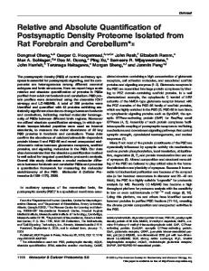
where B(· , ·) is the beta function, ξ1 , ξ2 , η2 > 0, η1 > −1, and r , which is the same in each component, is the estimate for the upper endpoint, given by r = ξ1 ξ2 . This distribution produced excellent fits to all the relative frame concentration measurements obtained from the seven datasets in Table I, and so will be used to evaluate the pdf convolution (18). A detailed discussion on the physical significance of the structure of the BGPD is given in Munro et al. (2003), along with full details of the fitting procedures used, and the effects of the poor resolution of the Lidar measurements. For given θ and X2 the right-hand side of (18) was estimated numerically using the trapezoidal rule, with the integrand being evaluated at the discrete relative locations x2 at which estimates of pr (θ; x2 ) were available. These estimates were available at 3-m intervals (roughly twice the spatial resolution of the Lidar) either side of x2 = 0, and within |x2 | L. (For example, L = 36 m for the mad14h data, and L = 60 m for the mad18a data.) A selection of results produced using this procedure, applied to the fits obtained from the mad14h and mad18a datasets, is illustrated in Figures 2 and 3 respectively, together with, for comparison, the histogram estimates for p (θ; X2 ) obtained from the corresponding absolute framework measurements. The results shown in Figure 2 are for the crossplume locations (X2 − µR ) = 0, ±21 m, and, in Figure 3, for (X2 − µR ) = 0, ±27 m. It is immediately evident from these plots that, at higher values of θ, the results of the convolution approximation produce excellent correspondence with the absolute frame pdfs generated from the measurements. However, at lower values of θ, the accuracy deteriorates as θ decreases. This characteristic was found at each crossplume location at which the convolution was performed and for all seven datasets analysed. This deterioration at low values of θ can be explained by the following. Since r (x2 ) generally decreased away from x2 = 0, then for θ > min , where min = min{r (x2 )} for −L x2 L, we have estimates for all non-zero values of pr (θ; x2 ) for −∞ < x2 < ∞. However, for θ < min this is not the case, and as θ decreases towards zero an increasing range of non-zero contributions to (18) will fall outside −L x2 L, and so will not be included in our approximation to the right-hand-side of (18). This problem becomes worse as |X2 − µR | increases, since then pˆ R (X2 − x2 ) gives increasing weight to the missing contributions to pˆ r (θ; x2 ). Thus, even if our models for pr (θ; x2 ) and pR (X2 −x2 ) are very good, we expect decreasing accuracy for p (θ; X2 ) as θ decreases below min and |X2 − µR | increases. Hence, to produce accurate estimates for p (θ; X2 ), at all values of θ, using the convolution (18), it is necessary to be able to prescribe pˆ r (θ; x2 ) at all locations x2 . This will inevitably involve considering the rate of approach of pr (θ; x2 ) to the limiting value δ(θ). Again, this needs much more analysis and will be discussed further in the final section.


265

Figure 2. Results of the convolution approximation, compared with the histograms plotted from the data, at the absolute framework positions (X2 − µR ) = 0, ±21 m from the mad14h dataset.

266

R. J. MUNRO ET AL.

Figure 3. Results of the convolution approximation, compared with the histograms plotted from the data, at the absolute framework positions (X2 − µR ) = 0, ±27 m from the mad18a dataset.


267

5.2. M OMENT CONVOLUTION For each of the seven datasets in Table I, the relative framework concentration measurements, at the discrete set of locations within |x2 | L, were used to gener(2) ate estimates for m(1) r (x2 ) and mr (x2 ). These estimates, along with the Gaussian estimates for pR (X2 ) obtained in Section 4, were then used to generate estimates for m(1) (X2 ) and m(2) (X2 ) by approximating the moment convolution (19). As with the pdf convolution, (18) was evaluated numerically for |X2 − µR | L using the trapezoidal rule at the discrete set of relative locations. In Section 1 the distinct differences between the statistical properties of (X, t) and r (x, t) were highlighted, i.e., the statistical properties of (X, t) are governed by the full spectrum of turbulence scales, and are thus subject to spatial smearing, whereas the statistical properties of r (x, t) are governed by the smaller scale turbulence with characteristic size of order, and smaller than, the instantaneous dimension of the plume, and are thus more characteristic of the in-plume concentration levels. A typical example of the degree of spatial smearing observed in the measurements is illustrated in Figure 4, which shows the estimated values, obtained from the mad14h absolute framework measurements, of m(1) and m(2) (thin solid (2) curves), together with the estimated values of m(1) r and mr (thin dashed curves), obtained from the relative framework measurements. (Note that the x2 values are aligned on the (X2 − µR ) axis so that x2 = 0 corresponds to (X2 − µR ) = 0.) The same degree of spatial smearing was also evident for the higher moments. For all (2) datasets analysed, the estimates m(1) r and mr were found to be symmetric about x2 = 0, and the rate of approach to the necessary limiting condition m(n) r (x2 ) → 0 (n) as |x2 | → ∞ was attained in the estimates mr (x2 ) at relatively small values of (2) x2 . Also, the estimates of m(1) r and mr were consistently found to have the smooth unimodal features characteristic of the examples shown in Figure 4. The results of the procedure used to estimate the moment convolution (19) (using the Gaussian estimates for pR (X2 )) are also shown in Figure 4 (bold solid curves). Comparing these with the corresponding estimates obtained from the measurements shows that the convolution procedure performs well, producing good correspondence at most locations |X2 − µR | L. Of course, as with the approximation used for the pdf convolution, there will be an associated error in the estimates produced. However, since for all datasets analysed, the limiting condition m(n) r (x2 ) → 0 is approximately attained in the estimates at locations within |x2 | L, this error will not have a significant effect, unlike the corresponding term for the pdf convolution procedure. In Figure 4, the estimates m(1) (X2 ) and m(2) (X2 ) generated directly from the mad14h absolute framework measurements appear to have a single subsidiary mode around (X2 − µR ) ≈ −40 m. Not surprisingly, given the smooth symmetric (2) unimodal behaviour of the estimates of m(1) r (x2 ) and mr (x2 ), and the Gaussian form used for pR (X2 ), this feature is not reproduced in the results of the convolution procedure. However, referring back to Figure 1 shows that, for the mad14h

268

R. J. MUNRO ET AL.

Figure 4. Plots comparing, for the mad14h dataset, the estimated values of m(1) and m(2) obtained using (i) the absolute framework measurements (thin solid curves), (ii) the convolution approximation (19) with Gaussian estimate for pR (bold solid curves), and (iii) the convolution (19) with (1) (2) KDE for pR (bold dashed curves). Also shown is the estimated values of mr and mr (thin dashed curves), obtained from the mad14h relative framework measurements.

data, the estimate pˆR (X2 ) obtained using the kernel density technique also has a subsidiary mode located at (X2 − µR ) ≈ −50 m. Therefore, the convolution approximation procedure was repeated for the mad14h data, this time with pˆ R (X2 ) obtained using the kernel density technique; the results are shown in Figure 4 (bold dashed curves). As expected, the results of this procedure agree more closely with the values generated from the data. For the majority of the datasets, the m(1) and m(2) generated directly from the measurements appear to agree well with a Gaussian form, and the corresponding estimates obtained using the convolution procedure (with Gaussian estimate for


269

pR ) produce very close fits. However, for some datasets, in particular those for which the kernel density procedure produced the least Gaussian-like estimates for pR (e.g., mad14h and flad23), the values of m(1) and m(2) obtained from the measurements have a structure similar to that illustrated in Figure 4.

6. Discussion In Section 4 the difficulties associated with analysing the plume centreline pdf were discussed, and, in particular, the shortcomings of the Risø Lidar measurements. Although the poor spatial resolution of these measurements will not significantly affect the accuracy of the measured values of R2 (t) obtained from the data, these one-dimensional measurements are clearly insufficient to provide an accurate analysis of the continuous vertical and horizontal displacement of the overall plume structure. However, with recent advances in Lidar technology, such as those already reported in the work of Bennett et al. (1992) and Bennett (1995), Lidar systems are now capable of scanning vertically up and down the plume cross section at a given downwind location. Measurements of this type would certainly reduce the errors caused by the imperfect spatial coverage of the one-dimensional Lidar measurements used in this analysis, allowing a much more accurate analysis of the complete centreline pdf pR (X) defined in (9). Furthermore, measurements of this type would also allow a more accurate analysis of the spatial variation of pr (θ; x) within the plume structure, and hence a full analysis of the general convolution relationships defined in (10) and (11). Modelling the absolute framework statistical quantities p (θ; X2 ) and m(n) (X2 ) using the convolution relationships defined in (10) and (11) effectively separates the dispersion process into two separate, essentially independent, components. That is, the relative dispersion of contaminant about the plume centreline position by turbulent motions of a universal form, and the random displacement of the plume governed by large-scale non-universal turbulence that depends on the overall geometry and boundary conditions of the flow and release. Separating the dispersion process in this way automatically incorporates essential physical properties that would not necessarily be directly addressed, or included, in any corresponding absolute framework modelling approach. In order that (18) can be used to provide applicable and accurate models for p (θ; X2 ) for all values of θ, it is necessary that pr (θ; x2 ) be prescribed for all values of x2 . This would require substantial quantities of quality data obtained over a wide range of meteorological and release conditions. In particular, the rate of approach of pr (θ; x2 ) to δ(θ) would need to be included to obtain reasonable accuracy at low values of θ. Of course, this would inevitably involve a degree of subjectivity since measurements at extreme ranges will not be available for validation.

270

R. J. MUNRO ET AL.

The implementation of the convolution (19) for the absolute framework moments m(n) (X2 ) is likely to be somewhat simpler. Firstly, because the relative framework moments m(n) r (x2 ) are likely to have a relatively simple structure, and hence should be reasonably easy to model accurately (for example using a Gaussian form). Secondly, because the necessary limiting condition m(n) r (x2 ) → 0 as |x2 | → ∞ is approximately attained at relatively short ranges, and so the corresponding subjectivity involved in modelling the values of m(n) r (x2 ) at large |x2 | will have little overall effect. The above features suggest that a sensible alternative approach to modelling p (θ; X2 ) could be the following. Firstly, assume a physically based parametric form for pˆ (θ; X2 ), which is known to compare well with absolute framework concentration measurements, e.g., the three-parameter exponential and generalized Pareto distribution of Lewis and Chatwin (1997). Then, for such a three-parameter (2) (3) model, using models for m(1) r (x2 ), mr (x2 ), mr (x2 ) and pR (X2 ), the corresponding models for m(1) (X2 ), m(2) (X2 ), m(3) (X2 ) could be generated using (19). Finally, these could then be used to model the behaviour of the parameters of the chosen form of pˆ (θ; X2 ) at any location X2 .

Acknowledgements This work was supported by the CEC funded COFIN project, contract number ENV4-CT97-0629. We would like to thank Hans Jørgensen, Torben Mikkelsen, Morten Nielsen and Søren Ott of Risø for useful comments and suggestions.

References Batchelor, G. K.: 1950, ‘The Application of the Similarity Theory of Turbulence to Atmospheric Diffusion’, Quart. J. Roy. Meteorol. Soc. 76, 133–146. Batchelor, G. K.: 1952, ‘The Effect of Homogeneous Turbulence on Material Lines and Surfaces’, Proc. Roy. Soc. A213, 349–366. Batchelor, G. K.: 1953, The Theory of Homogeneous Turbulence, Cambridge University Press, Cambridge, 197 pp. Bennett, M.: 1995, ‘A Lidar Study of the Limits to Buoyant Plume Rise in a Well-Mixed Boundary Layer’, Atmos. Environ. 29, 2423–2288. Bennett, M., Sutton, S., and Gardiner, D. R. C.: 1992, ‘An Analysis of Lidar Measurements of Buoyant Plume Rise and Dispersion at Five Power Stations’, Atmos. Environ. 26, 3249–3263. Chatwin, P. C.: 1990, ‘Statistical Methods for Assessing Hazards Due to Dispersing Gases’, Environmetrics 1, 143–162. Chatwin, P. C. and Sullivan, P. J.: 1979a, ‘The Relative Diffusion of a Cloud of Passive Contaminant in Incompressible Turbulent Flow’, J. Fluid Mech. 91, 337–355. Chatwin, P. C. and Sullivan, P. J.: 1979b, ‘Measurements of Concentration Fluctuations in Relative Turbulent Diffusion’, J. Fluid Mech. 94, 83–101. Chatwin, P. C., Lewis, D. M., and Sullivan, P. J.: 1995, ‘Turbulent Dispersion and the Beta Distribution’, Environmetrics 6, 395–402.


271

Gifford, F.: 1959, ‘Statistical Properties of a Fluctuating Plume Dispersion Model’, Adv. Geophys. 6, 117–137. Lewis, D. M. and Chatwin, P. C.: 1995, ‘The Treatment of Atmospheric Dispersion Data in the Presence of Noise and Baseline Drift’, Boundary-Layer Meteorol. 72, 53–85. Lewis, D. M. and Chatwin, P. C.: 1997, ‘A Three-Parameter pdf for the Concentration of an Atmospheric Pollutant’, J. Appl. Meteor. 36, 1064–1075. Measures, R. M.: 1984, Laser Remote Sensing – Fundamentals and Applications, John Wiley and Sons Ltd., 510 pp. Mikkelsen, T., Jørgensen, H. E., Thykier-Nielsen, S., Lund, S. W., and Santabarbara, J. M.: 1995, Final Data and Analysis Report on: High-Resolution in Plume Concentration Fluctuations Measurements Using Lidar Remote Sensing Technique, Technical Report No. Risø-R-852(EN), Risø National Laboratory, Roskilde, Denmark. Munro, R. J., Chatwin, P. C., and Mole, N.: 2003, ‘A Concentration pdf for the Relative Dispersion of a Contaminant Plume in the Atmosphere’, Boundary-Layer Meteorol. 106, 411–436. Mylne, K. R. and Mason, P. J.: 1991, ‘Concentration Fluctuation Measurements in a Dispersing Plume at a Range of Up to 1000 m’, Quart. J. Roy. Meteorol. Soc. 117, 177–206. Narayan, R. and Nityananda, R.: 1986, ‘Maximum Entropy Image Restoration in Astronomy’, Annu. Rev. Astron. Astrophys. 24, 127–170. Nielsen, M., Ott, S., Jørgensen, H. E., Bengtsson, R., Nyren, K., Winter, S., Ride, D., and Jones, C.: 1997, ‘Field Experiments with Dispersion of Pressure Liquefied Ammonia’, J. Hazard. Mater. 56, 59–105. Reynolds, A. M.: 2000, ‘Representation of Internal Plume Structure in Gifford’s Meandering Plume Model’, Atmos. Environ. 34, 2539–2545. Roussas, G. G.: 1997, A Course in Mathematical Statistics, 2nd edn., Academic Press, 572 pp. Sullivan, P. J.: 1990, ‘Physical Modelling of Contaminant Diffusion in Environmental Flows’, Environmetrics 1, 163–177. Yee, E. and Wilson, D. J.: 2000, ‘A Comparison of the Detailed Structure in Dispersing Tracer Plumes Measured in Grid-Generated Turbulence with a Meandering Plume Model Incorporating Internal Fluctuations’, Boundary-Layer Meteorol. 94, 253–296.