Some simulations of the effect of varying excitation parameters on the transients of reed instruments Fabrice Silva, Philippe Guillemain, Jean Kergomard, Christophe Vergez, Vincent Debut
To cite this version: Fabrice Silva, Philippe Guillemain, Jean Kergomard, Christophe Vergez, Vincent Debut. Some simulations of the effect of varying excitation parameters on the transients of reed instruments. 2013.
HAL Id: hal-00779636 https://hal.archives-ouvertes.fr/hal-00779636 Submitted on 22 Jan 2013
HAL is a multi-disciplinary open access archive for the deposit and dissemination of scientific research documents, whether they are published or not. The documents may come from teaching and research institutions in France or abroad, or from public or private research centers.
L’archive ouverte pluridisciplinaire HAL, est destin´ee au d´epˆot et `a la diffusion de documents scientifiques de niveau recherche, publi´es ou non, ´emanant des ´etablissements d’enseignement et de recherche fran¸cais ou ´etrangers, des laboratoires publics ou priv´es.
Some simulations of the effect of varying excitation parameters on the transients of reed instruments F. Silva, Ph. Guillemain, J. Kergomard and Ch. Vergez∗ LMA, CNRS, UPR 7051, Aix-Marseille Univ., Centrale Marseille F-13402 Marseille cedex 20, France. V. Debut † Applied Dynamics Laboratory, Campus Tecnológico e Nuclear, Instituto Superior Técnico/Universidade Técnica de Lisboa, 2686-953 Sacavem, Portugal. January 22, 2013
Abstract This paper considers the simulation of self-sustained oscillations in reed and brass instruments, based on a compact continuous-time formulation of the sound production mechanism. The control parameters such as the mouth pressure and the player’s embouchure, but also the acoustic resonator and the reed may vary with respect to time, allowing the analysis of transient and non-stationary phenomena like changes of regime. A particular attention is first given to staccato notes, with comparison of the evolution of the instantaneous frequency in simulations to theoretical and experimental results. This shows the importance of using realistic control parameters on the onset of the oscillations. When the acoustic resonator is modelled using a modal expansion with non-stationary resonance frequencies and damping, it is also possible to simulate and study slurs and musical effects like the wah-wah, gaining some insight on the mechanisms involved.
1
Introduction
In sound analysis or synthesis, transients are necessary in the sense that they carry information useful to listener to identify the instrument and to perceive the musician intention. Time-domain simulation is helpful in understanding the relation between variation in control parameters and characteristics of the resulting sound. The present paper considers the time-domain simulation using modal expansion for the behaviour of the passive parts of the reed instruments, i.e. the reed and the resonator (the nonlinear part corresponding to the coupling between airflow and the reed acting as a valve). This allows taking into account in a simple way the variation of the control parameters, such as the mouth pressure and the player’s embouchure, but also the acoustic resonator and the reed whose parameters may vary with respect to time, allowing the analysis of transient and non-stationary phenomena like changes of regime. In the assumption of linear acoustics, a resonator can be fully described by its input impedance, and this quantity can be expanded into modes of the resonator. This leads to the solving of a set of Ordinary Differential Equations. Modal analysis is widely used in musical acoustics to analyse and reproduce the vibration of complex vibrating structures, but few applications have been treated for self-sustained instruments (Ref. [1] for the study of the bowed string, Ref. [2] for sound synthesis, and Ref. [3] for a dynamical system approach). ∗ {silva,vergez,guillemain,kergomard}@lma.cnrs-mrs.fr †
[email protected]
1
We first present the modelling of the problem, based upon a classical description of the different parts of the instrument, then the time domain simulation as performed within the Moreesc tool [4], and present two examples: the first one is the mouth pressure rises in clarinet-like instrument, and the effect of the speed of the rise on the resulting attack. The second one concerns brass instruments, first slurred transients obtained when the natural frequencies of the lips are varying during the sound for a given length of the resonator, then the wah-wah effect simulating dynamic variation of the input impedance of the trumpet.
2
Modelling
The elementary model used by many authors (see e.g. [5]) assumes the representation of the sound production mechanism by an acoustic resonator and an exciter, and their mutual coupling. This leads to a system of three equations modelling the reed (cane or lip reed) motion, the acoustic waves in the bore of the instrument and the flow of air through the reed channel. Those are formulated using a control-theory approach, defining a state vector X ( t) and its dynamics d X / dt = f ( X , t, . . .). Hereafter are described the partial state vector associated with each part of the system: £ ¤T X = X r, X a, X f .
2.1
(1)
Reed motion
Extending previous models such as the massless reed [6] or the single d.o.f. [7], a general class of transfer function is considered, relating the reed channel opening h( t) to the driving term, here the pressure difference ∆ p( t):
dN h dt N
. . . + a N −1
dh d∆ p dM∆p + a N ( h( t) − h 0 ) = b 0 + . . . + b M −1 + b M ∆ p ( t) dt dt dt M
(2)
with M ≤ N , or, using the Laplace transform PM b m s M −m H ( s) = PmN=0 N −n ∆ P ( s) n=0 a n s
(3)
where s is the Laplace variable (usually evaluated on the frequency axis s = j ω), and a 0 = 1. This simplifies for the single d.o.f. reed with natural angular frequency ωr , damping q r and stiffness K r to N = 2, M = 0 and a 1 = q r ωr , a 2 = ω2r and b 0 = ω2r /K r . The observable canonical form is adopted, with the partial state vector: · ¸T dh d N −1 h X r = h ( t ), , . . . , N −1 . dt dt
(4)
Note also that refinements such as beating reed are handled using contact forces as additional driving terms.
2.2
Acoustic resonator
While it is possible to fine-grainly describe the pecularities of the geometry and of the phenomena at the open tone holes or at the bell, the focus is here given to the results of those on the input impedance of the bore. This approach is valid since the valve-bore coupling is localised at the entrance of the bore. Furthermore, the input impedance is parametrised in order to avoid convolution with a long tailed impulse response. The mouthpiece pressure p( t) is expanded as a sum of components p n ( t) defined by the modal expansion of the input impedance:
Z e ( s) =
X P ( s) X C n d pn = ⇔ p( t) = p n ( t) with = C n u( t) + s n p n ( t). U ( s) dt n s − sn n
2
(5)
Poles s n and residues C n can be derived analytically for simple models [8], from numerical identification on a measured input impedance or estimated through a spatial modal analysis (with observation at the bore entrance). Hermitian symmetry implies real or complex conjugates poles (and residues), so that X X 2 ℜe ( p n ( t)) + p n ( t ). (6) p ( t) = s n ∈R
ℑm( s n ) >0
The partial state vector thus contains the components p n ( t) such that ℑm ( s n ( t)) ≥ 0, and its dynamics is given by Eq. (5).
2.3
Airflow
According to Hirchberg [6], the airflow through the reed channel u( t) can be described by a stationnary expression based on the Bernoulli theorem: s
u ( t) = h( t)
2∆ p( t) ρ
(7)
with ρ the air density. Within this approximation, the flow rate u( t) is a simple observable so that the partial state vector related to fluid mechanics is empty. Reed motion induced flow only adds a term in the previous expression, and a partial state vector X f l appears if an instationnary flow description is considered.
3 3.1
Time-domain simulation ODE integration
Eqs. (2), (5) and (7) define a continuous-time formulation that do not require to be transposed to the discrete-time domain. In fact a wide family of Ordinary Differential Equations (ODE) solvers are able to handle such a formulation, allowing extra precautions when approching singular points such as instants when the system becomes stiff or leaves this property. When considering stability of the scheme, the adaptative step-size and/or order-size provide a deep advantage in comparison with fixed step-size scheme like Euler method for instance. The following integrators have been tested in the present study: Explicit Euler method: the bounded stability region requires small time steps. For usual audio sampling frequencies, this condition forbids the explicit single-step method, leading to instability and explosion of the computed solution. Practically, the sampling frequency can be increased (by a factor M ), it is quite usual for the time step to be about 0.01/ f s ( M = 100 intermediate steps between samples at the usual audio sampling frequency f s = 44.1 kHz). The result is then obtained discarding the intermediate steps, as in the following Runge-Kutta methods. Explicit Runge-Kutta methods of order 5(4) and 8(5,3) perform adaptive step size to bound the local truncation error. As in the Euler integrator, the intermediate steps used to obtain the high order are discarded. VODE and LSODA are multistep methods that re-use previous steps to gain efficiency instead of computing and discarding intermediate steps. They are also variable-order and adaptive step size, and can use both implicit Adams-Moulton methods (AM) or Backward differentiation formulas (BDF) depending on whether the problem is locally stiff or not. LSODA has the advantage of automatically performing the switch between the two methods when stiffness has been detected.
3.2
Time-varying control parameters
Simulation requires that the control parameters are not oversimplified in order for the results to sound perceptively natural. As noted in [9] and also in [10] on clarinet and [11] on brass instruments, it is essential to understand how to perform starting transients and transition
3
between slurred notes. The current code has been designed to allow the definition of timevariable mouth pressure and reed channel opening at rest, but also to dynamically change the reed transfer function and the input impedance using coefficients a n and b m , poles s n and residues C n that are allowed to change with respect to time. This involves using academic profiles such as step or smoothed steps, measured mouth pressure or even interpolation between two configurations of the acoustic resonator. The continuous-time domain formulation is preserved through the approximation of sampled signals by cubic spline if needed. Results below will present a few simulations using this process.
4
Results
4.1
Mouth pressure rise and quality of the attack
Previous studies [12, 13] showed how the time needed for setting the mouth pressure to its steady value affects the oscillation growth. For slow rise (about 10 ms), there is an exponential growth of the fundamental frequency partial that only transfers some energy to the higher harmonics when saturating (i.e. when the nonlinearity of the airflow relationship gets involved). On the contrary, the quickly rising input (less than 1 ms) distributes energy amongst all the resonances before mode-locking ensures reorganisation into partials, as shown by Debut [12] defining master and slave components. These results are extended here by simulating the attack of a 50 cm long cylinder mode (with radius 7 mm, truncated to 8 modes) with a cane reed (ωr = 2π × 1.5 kHz, q r = .4 and K r = 0.5 GPa/m2 , aperture at rest 7 mm2 ) for mouth pressure growing Pa with Pression bouche from 0 to 1708 Pression bec various rise time. /
Amplitude (kPa)
/
1 ms 2 ms 5 ms 10 ms
102 101 100 5 ms 10 1 10 ms 10 2 20 ms 10 3 10 4 10 5 50 ms 10 6 ms 10 7 100 200 ms 10 80.0 0.2 0.4
0.6
0.8
1.0
30 Deviation (cents)
20 ms 50 ms 100 ms 200 ms 0.0
0.2
0.4
(s)
0.6
0.8
1.0
20 10 0 10 20 300 10 20 30 40 50 60 70 80 time (ms)
Figure 1: Starting transients for various rise time of the mouth pressure. Left: blue curves for input pressure signal, red curve for mouth pressure. Upper right: amplitude of signals. Lower right: oscillation frequency deviation to steady-state frequency (same colors as for the upper right axes, quickly rising mouth pressure only). F e = 44.1 kHz. Signals on Fig. 1 show an apparent delay in the start of the sound for rise times greater than 5 ms. However, the amplitude extraction evidences that all oscillations have exponential growth with a time constant independant of the rise time before reaching the steady state.
4
Note that the latter seems also to be the same for all the simulations, even for smaller rise time. In his PhD thesis [12], Debut explained why the frequency is not the same during the very short time when the functioning can be regarded as linear, and during the steady-state regime. For the former, the eigenfrequencies differ from the eigenfrequencies of the passive resonator due to the energy supply at the input of the bore, and can be much higher if the sudden increase of the mouth pressure is large. The result shown in Fig. 1 (lower right axes) is in accordance with the work by Debut (Ref. [12], page 109): for the most sudden attack, the instantaneous frequency starts with more than 20 cents above the steady-state frequency. The oscillation frequency then evolves when the harmonics fit into the multimodal resonator, explained as the mode locking phenomenon by Ref. [14]. Concerning oscillations occurring during the first 60 milliseconds, they are due to the analysis method. It is well known that instantaneous frequency estimation on nonstationary multi-components signals is a tricky problem that combines the choice of the time-frequency analysis window and the speed of variations of amplitude and frequency modulation laws. However several questions can be asked about this frequency variation. Preliminary experimental studies have been done with professional clarinettists. They exhibit a similar tendency, i.e. in general the instantaneous frequency decreases during the first milliseconds, but sometimes, it increases. Obviously many other reasons can be sought than the previous one. As an example, the tuning control by the instrumentalist can be the main reason of this behaviour, but this remains to be investigated. Moreover the perceptive effect of this variation is not known, and it is not sure that it is important, because the duration is very short. Further work is needed.
4.2
Slurred transients in brass instruments
The slurred transients are investigated simulating the sound production when increasing and decreasing the natural frequency of the lips of a brass musician. The measured input impedance of a Yamaha YTR1335 trumpet has been expanded on 12 modes, with a parametrisation error less than 2% (see Fig. 2).
Modal Measured
arg(Z)
|
Z|
70 60 50 40 30 20 10 0 ◦ 90 45 ◦ 0◦ -45 ◦ -90 ◦ 0
500
1000
f (Hz)
1500
2000
Figure 2: Measured input impedance of the trumpet and modal expansion. For a linear decrease from 1 kHz to 100 Hz of the natural frequency of the lips (modelled as a single d.o.f. oscillator with q r = 0.1 and K r = 0.8 GPa/m2 ), downwards slurs are observed (see Fig. 3, red curves) when the lips resonance frequency goes too far beyond each of the acoustic resonance frequencies. These changes of regime define playing frequency ranges that are almost centered on the resonance frequencies of the bore (±50cents). On the contrary, upwards slurred transients happen when ωr crosses one of the bore resonances, i.e. leading to sharper notes. This is what is expected when focusing on oscillation threshold (see e.g. [15]). This difference between the behaviors of the upwards and downwards slurred transients corresponds to the feeling of the musician when practising three-notes (up then down, or down
5
then up), requiring important changes on the lips tension. Another consequence is that the musician has to adopt some strategy to overcome the sharper note obtained on upward slur.
(a)
f
A#4
fac7
G4
fac6
fac4
downwards upwards
E4 fac5
fac6
fLips
fac7
(b)
100
C5
fac8
fac5
150
D5
dev(f) (cents)
fac9
fac8
50 E4
G4
0
C5
A#4
-50
downwards upwards
-100 -150 4
fac9
D5
fac5
fac
fac6
fLips
fac8
fac7
fac9
2
Figure 3: Upward (red curves) and downward (black 1 curves) slurs of a trumpet. No valve change, linear variation of ωr . Dotted lines are the acoustic resonances frequencies. 0
˜p(t)
It is also interesting to investigate how the 1change of regime takes place. In Fig. 4, the lower step of the mouthpiece pressure signal seems to lose stability, like an unstable amplitude modulation until the slur occurs and the 2amplitude modulation vanishes too, leading to the flatter note. Comparison with the phenomena presented by two players in Ref. [11] 3 requires further investigation on the strategies adopted by these musicians. 4 2 600 1 550
f (Hz)
˜p(t)
0 1 2
500
3 4 600
450 6.25
6.30
6.35
t (s)
6.40
6.45
6.50
f (Hz)
Figure 4: Zoom on a downward slur of a trumpet: time-domain signal and instantaneous fre550 quency. 500
4.3
Wah-wah effect
Last result focuses on the wah-wah effect on the trumpet. Using a rubber plunger mute at 450 several6.30 distances 6.25 6.35 from 6.40the bell, 6.45 a series 6.50 of four input impedance measurements has been t (s) allowing to define trajectories for each of the poles and residues. Arexpanded onto modes, bitrary 2 s-long sequences of closing and opening of the bell have been modelled as shown in Fig. 5 (left axes, solid curves are trajectories of the modulus of the poles). Simulation for time-invariant characteristics of the lips (ωr = 2π × 500 Hz, q r = 0.1, K r = 0.8 GPa/m2 ) leads to sound production with instantaneous frequency oscillating over a range of 20 cents (dashed curve in Fig. 5, left axes). The main effect is visible on the amplitude modulation (Fig. 5, upper right axes), and on the spectral centroïd frequency (Fig. 5, lower right axes), leading to perceptible variations of the loudness and timbre.
6
20
Mute closing the bell
SCF (kHz) Amplitude (dB)
dev(f) (cents)
30
Mute closing the bell
10 Mute far from the bell
0 10
fosc ω2
2
ω3 ω4
ω5 ω6
3
t (s)
ω7 ω8
ω9
4
0 1 2 3 4 5 2.1 2.0 1.9 1.8 1.7 1.6 2
3
t (s)
4
Figure 5: Deviation, amplitude and spectral centroïd frequency for the wah-wah effect simulation.
References [1] J. Antunes, M. G. Tafasca, and L. L. Henrique, “Simulation of the bowed-string dynamics-part 1- a nonlinear modal approach”, in Actes du 5ème congrès français d’acoustique, 285–288 (2000). [2] R. E. Caussé, J. Bensoam, and N. Ellis, “Modalys, a physical modeling synthesizer: More than twenty years of researches, developments, and musical uses”, in 162nd Meet. Acous. Soc. Am. (2011). [3] A. Barjau and V. Gibiat, “Study of woodwind-like systems through nonlinear differential equations. part ii. real geometry”, J. Acous. Soc. Am. 102, 3032–3037 (1997). [4] F. Silva, Ch. Vergez, J. Kergomard and Ph. Guillemain, “Moreesc : Modal Resonator - Reed Interaction Simulation Code”, URL http://moreesc.lma.cnrs-mrs.fr/, (last accessed on jan. 21th, 2013). [5] A. Chaigne and J. Kergomard, Acoustique des instruments de musique (Belin) (2008). [6] A. Hirschberg, J. Kergomard, and G. Weinreich, eds., Mechanics of Musical Instruments, CISM Courses and Lectures No.355 (Springer-Verlag, Wien - New York) (1995). [7] T. A. Wilson and G. S. Beavers, “Operating modes of the clarinet”, J. Acous. Soc. Am. 56, 653–658 (1974). [8] F. Silva, “Émergence des auto-oscillations dans un instrument de musique à anche simple”, Ph.D. thesis, Aix Marseille University (2009). [9] J. M. Grey, “Multidimensional perceptual scaling of musical timbres”, J. Acous. Soc. Am. 61, 1270–1277 (1977). [10] P. Guillemain and A. Merer, “Rôles du contrôle et du timbre dans la perception du naturel de sons de clarinette”, in 10ème Congrès Français d’Acoustique, (2010). [11] S. Logie, P. Chick, John, S. Stevenson, and M. Campbell, “Upward and downward slurred transients on brass instruments: Why is one not simply the inverse of the other?”, in 10ème Congrès Français d’Acoustique, (2010). [12] V. Debut, “Deux études d’un instrument de musique de type clarinette : analyse des fréquences propres du résonateur et calcul des auto-oscillations par décomposition modale”, Ph.D. thesis, Université de la Méditerranée - Aix-Marseille II (2004). [13] F. Silva, V. Debut, J. Kergomard, C. Vergez, A. Deblevid, and P. Guillemain, “Simulation of single reed instruments oscilations based on modal decomposition of bore and reed dynamics”, in Proceedings of the International Congress of Acoustics (Espagne Madrid), (2007). [14] N. H. Fletcher, “Mode locking in nonlinearly excited inharmonic musical oscillators”, J. Acous. Soc. Am. 64, 1566–1569 (1978). [15] J. S. Cullen, J. Gilbert, and D. M. Campbell, “Brass instruments: Linear stability analysis and experiments with an artificial mouth”, Acta Acustica united with Acustica 86, 704–724 (2000).
7