Mar 20, 2013 - William of Ockham was a English Franciscan friar of the 14th century. ...... eralization of the corresponding Chi-Square goodness-of-fit test in several ...... health economics, planning of public transportation, evaluation of public ...
Some (statistical) applications of Ockham’s principle Erwan Le Pennec
To cite this version: Erwan Le Pennec. Some (statistical) applications of Ockham’s principle. Statistics [math.ST]. Universit´e Paris Sud - Paris XI, 2013.
HAL Id: tel-00802653 https://tel.archives-ouvertes.fr/tel-00802653 Submitted on 20 Mar 2013
HAL is a multi-disciplinary open access archive for the deposit and dissemination of scientific research documents, whether they are published or not. The documents may come from teaching and research institutions in France or abroad, or from public or private research centers.
L’archive ouverte pluridisciplinaire HAL, est destin´ee au d´epˆot et `a la diffusion de documents scientifiques de niveau recherche, publi´es ou non, ´emanant des ´etablissements d’enseignement et de recherche fran¸cais ou ´etrangers, des laboratoires publics ou priv´es.
Habilitation à Diriger des Recherches
Some (statistical) applications of Ockham’s principle
Erwan Le Pennec
Soutenue le 19 mars 2013
Devant le jury constitué de:
G. Celeux, A. Juditsky, S. Mallat, P. Massart, D. Picard, A. Trouvé,
Directeur de recherche, Professeur, Professeur, Professeur, Professeur, Professeur,
Select - Inria / LMO - Université Paris Sud Laboratoire J. Kuntzmann - Université Joseph Fourier (rapporteur) DI - ENS Ulm LMO - Université Paris Sud / Select - Inria (rapporteur) LPMA - Université Paris Diderot CMLA - ENS Cachan (rapporteur)
2
3
Numquam ponenda est pluralitas sine necessitate Plurality must never be posited without necessity William of Ockham (c. 1288 – c. 1348)
William of Ockham was a English Franciscan friar of the 14th century. He was also a scholastic philosopher which is often credited for the law of parsimony that states roughly that among good explanations one should favor the simplest ones. Although he was not the first to postulate this principle of simplicity, this idea can be traced back to Aristotle, his name is now associated to this idea which is often called Ockham’s principle or Ockham’s razor. I would not consider this principle as a philosophical doctrine but rather as a loose heuristic principle used in sciences: a good solution is often obtained by balancing its apparent goodness and its complexity. Although very naive, this principle turns out to be the cornerstone of my scientific contributions. For sure, we will have to specify definitions for good solution, apparent goodness and complexity, but it is nevertheless amusing to me that up to some technicalities this simple idea summarizes most of my works.
4
Contents 0 Survol . . . . . . . . . . . . . . . . . . . . . . . . . . . . . . . . . . 1 Estimating the mean of a Gaussian: a toy example . . . . . . . . . 1.1 Trivial estimate and James-Stein’s one . . . . . . . . . . . . . 1.2 Projection based estimator . . . . . . . . . . . . . . . . . . . . 1.3 Model selection and thresholding . . . . . . . . . . . . . . . . 1.4 Importance of the basis . . . . . . . . . . . . . . . . . . . . . . 1.5 Basis choice . . . . . . . . . . . . . . . . . . . . . . . . . . . . 1.6 What’s next? . . . . . . . . . . . . . . . . . . . . . . . . . . . 2 Overview . . . . . . . . . . . . . . . . . . . . . . . . . . . . . . . . 2.1 Brief overview . . . . . . . . . . . . . . . . . . . . . . . . . . . 2.2 Manuscript organization . . . . . . . . . . . . . . . . . . . . . 2.2.1 A chronological point of view? . . . . . . . . . . . . . . . 2.2.2 An approximation theory point of view? . . . . . . . . . 2.2.3 A Statistical point of view! . . . . . . . . . . . . . . . . 3 Estimation in the white noise model . . . . . . . . . . . . . . . . . 3.1 Image acquisition and white noise model . . . . . . . . . . . . 3.2 Projection Estimator and Model Selection . . . . . . . . . . . 3.2.1 Approximation space VN and further projection . . . . . 3.2.2 Model selection in a single orthonormal basis . . . . . . 3.2.3 Model Selection in a dictionary of orthonormal bases . . 3.3 Best basis image estimation and bandlets . . . . . . . . . . . . 3.3.1 Minimax risk and geometrically regular images . . . . . 3.3.2 Estimation in a single basis . . . . . . . . . . . . . . . . 3.3.3 Estimation in a fixed frame . . . . . . . . . . . . . . . . 3.3.4 Dictionary of orthogonal bandlet bases . . . . . . . . . . 3.3.5 Approximation in bandlet dictionaries . . . . . . . . . . 3.3.6 Bandlet estimators . . . . . . . . . . . . . . . . . . . . . 3.4 Maxiset of model selection . . . . . . . . . . . . . . . . . . . . 3.4.1 Model selection procedures . . . . . . . . . . . . . . . . 3.4.2 The maxiset point of view . . . . . . . . . . . . . . . . . 3.4.3 Abstract maxiset results . . . . . . . . . . . . . . . . . . 3.4.4 Comparisons of model selection estimators . . . . . . . . 3.5 Inverse problem, needlet and thresholding . . . . . . . . . . . 3.5.1 Inverse problem, SVD and needlets . . . . . . . . . . . . 3.5.2 A needlet based inversion for Radon transform . . . . . 3.5.3 A needlet based inversion for Radon transform of axially 3.6 Recreation: NL-Means and aggregation . . . . . . . . . . . . . 3.6.1 Image denoising, kernel and patch methods . . . . . . . 3.6.2 Aggregation and the PAC-Bayesian approach . . . . . . 3.6.3 Stein Unbiased Risk Estimator and Error bound . . . . 3.6.4 Priors and numerical aspects of aggregation . . . . . . . 5
. . . . . . . . . . . . . . . . . . . . . . . . . . . . . . . . . . . . . . . . . . . . . . . . . . . . . . . . . . . . . . . . . . . . . . . . . . . . . . . . . . . . . . . . . . . . . . . . . . . . . . . . . . . . . . . . . . . . . . . . . . . . . . . . . . . . . . . . . . . . . . . . . . . . . . . . . . . . . . . . . . . . . . . . . . . . . . . . . . . . . . . . . . . . . . . . . . . . . . . . . . . . . . . . . . . . . . . . . . . . . . . . . . . . . . . . . . . . . . . . . . . . . . . . . . . . . . . . . . . . . . . . . . . . . . . . . . . . . . . . . . . . . . . . . . . . . . . . . . . . . . . . . . . . . . . . . . . . . . . . . . . . . . . . . . . . . . . . . . . . . . . . . . . . . . . . . . . . . . . . . . . . . . . . . . . . . . . . . . . . . . . . . symmetric objects . . . . . . . . . . . . . . . . . . . . . . . . . . . . . . . . . . . . . . . . . . . . . . . . . . . . . . .
. . . . . . . . . . . . . . . . . . . . . . . . . . . . . . . . . . . . . . . . .
. . . . . . . . . . . . . . . . . . . . . . . . . . . . . . . . . . . . . . . . .
. . . . . . . . . . . . . . . . . . . . . . . . . . . . . . . . . . . . . . . . .
. . . . . . . . . . . . . . . . . . . . . . . . . . . . . . . . . . . . . . . . .
. . . . . . . . . . . . . . . . . . . . . . . . . . . . . . . . . . . . . . . . .
. . . . . . . . . . . . . . . . . . . . . . . . . . . . . . . . . . . . . . . . .
7 9 9 9 10 11 12 12 13 13 15 15 16 17 21 21 22 22 22 24 25 25 26 27 28 29 30 31 33 34 36 39 43 44 47 53 58 59 61 62 63
6
4 Density estimation . . . . . . . . . . . . . . . . . . . . . . . . . . . . . . . . . . . . 4.1 Density estimation . . . . . . . . . . . . . . . . . . . . . . . . . . . . . . . . . 4.2 Dictionary, adaptive threshold and `1 penalization . . . . . . . . . . . . . . . . 4.2.1 Dictionary, Lasso and Dantzig . . . . . . . . . . . . . . . . . . . . . . . . 4.2.2 The Dantzig estimator of the density s0 . . . . . . . . . . . . . . . . . . 4.2.3 Results for the Dantzig estimators . . . . . . . . . . . . . . . . . . . . . 4.2.4 Connections between the Dantzig and Lasso estimates . . . . . . . . . . 4.2.5 Calibration . . . . . . . . . . . . . . . . . . . . . . . . . . . . . . . . . . 4.3 Copula estimation by wavelet thresholding . . . . . . . . . . . . . . . . . . . . 4.3.1 Estimation procedures . . . . . . . . . . . . . . . . . . . . . . . . . . . . 4.3.2 Minimax Results . . . . . . . . . . . . . . . . . . . . . . . . . . . . . . . 4.3.3 Maxiset Results . . . . . . . . . . . . . . . . . . . . . . . . . . . . . . . . 5 Conditional density estimation . . . . . . . . . . . . . . . . . . . . . . . . . . . . . 5.1 Conditional density, maximum likelihood and model selection . . . . . . . . . 5.2 Single model maximum likelihood estimate . . . . . . . . . . . . . . . . . . . . 5.2.1 Asymptotic analysis of a parametric model . . . . . . . . . . . . . . . . 5.2.2 Jensen-Kullback-Leibler divergence and bracketing entropy . . . . . . . 5.2.3 Single model maximum likelihood estimation . . . . . . . . . . . . . . . 5.3 Model selection and penalized maximum likelihood . . . . . . . . . . . . . . . 5.3.1 Framework . . . . . . . . . . . . . . . . . . . . . . . . . . . . . . . . . . 5.3.2 A general theorem for penalized maximum likelihood conditional density 5.4 Partition-based conditional density models . . . . . . . . . . . . . . . . . . . . 5.4.1 Covariate partitioning and conditional density estimation . . . . . . . . 5.4.2 Piecewise polynomial conditional density estimation . . . . . . . . . . . 5.4.3 Spatial Gaussian mixtures, models, bracketing entropy and penalties . . 5.5 Binary choice model . . . . . . . . . . . . . . . . . . . . . . . . . . . . . . . . 6 Conclusion . . . . . . . . . . . . . . . . . . . . . . . . . . . . . . . . . . . . . . . . A Let It Wave . . . . . . . . . . . . . . . . . . . . . . . . . . . . . . . . . . . . . . .
CONTENTS
. . . . . . . . . . . . . . . . . . . . . . . . . . . . . . . . . . . . . . . . . . . . . . . . . . . . . . . . . . . . . . . . . . . . . . . . . . . . . . . . . . . . . . . . . . . . . . . . . . . . . . . . . . . . . . . . . . . . . . . . . . . . . . . . . . . . . . . . . . . . estimation . . . . . . . . . . . . . . . . . . . . . . . . . . . . . . . . . . . . . . . . . . . . . . . . .
. . . . . . . . . . . . . . . . . . . . . . . . . . . .
65 65 65 65 68 70 74 74 75 77 79 79 83 83 85 85 87 89 90 90 91 92 92 94 96 101 105 119
Chapitre 0
Survol Ce manuscrit décrit mon travail scientifique de ces dix dernières années. Celui peut-être découpé autour des dix thèmes suivants :
Thème 0. Bandelettes et approximations (2000-2005) Dans ce travail, qui correspond à ma thèse de doctorat réalisé sous la direction de S. Mallat, j’ai construit une nouvelle représentation d’image adaptée aux images géométriques : la représentation en bandelettes. Nous avons démontré que les propriétés d’approximation de ce frame adaptatif conduisait pour les images géométriques à des vitesses d’approximation non linéaires adaptatives à des termes logarithmique près. Ces résultats ont été transcrits en des résultats de compression à la fois théoriquement et numériquement.
Thème 1. Bandelettes et estimations (2002-2011) Profitant des propriétés d’approximations des bandelettes, nous avons proposé un premier algorithme de débruitage d’image basé sur le principe MDL (Comprimer c’est presque estimer). En utilisant ensuite les bases de bandelettes de seconde génération de G. Peyré, nous avons en collaboration avec Ch. Dossal utilisé les techniques de L. Birgé et P. Massart pour proposer un algorithme de sélection de modèles de bandelettes dont nous avons pu prouver la quasi optimalité minimax pour des images géométriques.
Thème 2. Maxiset (2004-2009) Une question naturelle est de se demander pour quelles fonctions l’estimateur précédent est-il efficace. Dans ce travail réalisé en collaboration avec F. Autin, J.-M. Loubes et V. Rivoirard, on montre que, sous des hypothèses faibles de structure, les fonctions bien estimées sont exactement celles bien approchées par des modèles de faibles dimensions de la collection.
Thème 3. Dantzig (2006-2010) En partant d’une question que nous a posée S. Tsybakov, j’ai étudié avec K. Bertin et V. Rivoirard une variation du Lasso dans un cadre d’estimation de densité. Nous avons pu calibrer de manière fine la pénalité de cet estimateur de Dantzig et vérifier théoriquement et numériquement ses performances.
Thème 4. Radon (2007-2012) En partant de la superbe construction de la représentation en needlet de P. Petrushev et des coauteurs, j’ai proposé avec G. Kerkyacharian et D. Picard une stratégie de seuillage en needlet pour inverser une transformée de Radon d’un objet dans le cadre du modèle du bruit blanc. Nous avons prouvé que cet estimateur est adaptatif et presque minimax pour une large gamme d’espace de Besov. Ces résultats ont été confirmés numériquement. En utilisant une construction similaire, j’ai obtenu en collaboration avec 7
8
CHAPITRE 0. SURVOL
M. Bergounioux et E. Trélat des résultats de type inégalité oracle pour la transformée de Radon d’objet axisymétrique.
Thème 5. Copule (2008-2009) Les stratégies de seuillage en ondelettes sont connues pour être efficaces. Dans ce travail avec F. Autin et K. Tribouley, nous montrons que c’est également le cas pour l’estimation des copules. Nous avons obtenu des estimateurs adaptatifs et quasi minimax pour les espaces de Besov. Ces résultats théoriques ont été confirmés par nos expériences numériques.
Thème 6. NL-Means (2008-2009) Ce travail correspond au début de la thèse de J. Salmon. Nous avons essayé d’étudier le lien entre l’une des méthodes numériques les plus efficaces de débruitage, les NL-means, et le principe statistique de pondération exponentielles. Notre analyse a conduit à des améliorations numériques publiées par J. Salmon.
Thème 7. Modèle du choix binaire (2010-2011) Dans ce travail avec E. Gautier, nous étudions un modèle classique économétrique : le modèle du choix binaire. Il s’agit d’un problème inverse qui se combine à une estimation de densité conditionnelle. Nous proposons une technique basé sur les ondelettes permettant d’obtenir des estimations adaptatives.
Thème 8. Segmentation d’image hyperspectrale (2010-2012) Une des techniques les plus classiques de classification non supervisée est basée sur des mélanges de gaussiennes dont les composantes sont associées à des classes. Avec S. Cohen, nous avons proposé une extension de ce modèle permettant de prendre en compte une covariable importante dans les images hyperspectrales, la position. Nous avons proposé un schéma numérique efficace qui nous a permis de tester avec succès notre algorithme sur des jeux de données réels venant de la plateforme IPANEMA du synchrotron Soleil.
Thème 9. Estimation de densité conditionnelle (2010-2012) L’algorithme précédent repose sur une estimation de densité par sélection de modèles. Nous avons cherché, et réussi, à le justifier théoriquement. Nous avons ainsi donné une nouvelle technique d’estimation de densité conditionnelle par maximum de vraisemblance pénalisé dont on contrôle l’efficacité sous des hypothèses faibles. L. Montuelle travaille sous notre direction sur des extensions du modèle de mélanges de gaussienne rentrant dans ce cadre. Après une introduction aux questions abordées à travers l’exemple jouet de l’estimation de la moyenne d’un vecteur gaussien, le manuscrit reprend, en anglais, la description de ces 10 thèmes. Il se concentre autour des thèmes de 1 à 9 en les organisant autour des modèles statistiques utilisés.
Chapter 1
Estimating the mean of a Gaussian: a toy example We focus in this first chapter on a very simple statistic problem: estimation of the mean of a Gaussian random vector of covariance matrix a known multiple of the identity. Let X ∈ RN be the unknown mean, this problem can be rewritten as the observation of Y = S + σW where W is a standard Gaussian vector and σ the known standard deviation. Our goal is now to estimate S from the observation Y .
1.1
Trivial estimate and James-Stein’s one
b = Y itself. This is indeed an unbiased The most natural estimate is the trivial one: one estimates S by S estimate which seems the best possible without any further assumptions. Using the quadratic risk, which corresponds here to the Kullback-Leibler risk up to the variance factor, as a good solution criterion, we obtain a goodness of h
i
b 2 = E kS − Y k2 = σ 2 N. E kS − Sk �
�
Is this the best one can do? No, as proved first by James and Stein [JS61]. They proposed to shrink toward 0 the previous estimate using
bJS = S
� 1−
(N − 2)σ 2 kY k2
� Y +
and have shown that as soon as n ≥ 3 this estimate always has a smaller quadratic risk than the trivial −2)σ 2 one. Heuristically, the shrinkage reduces the variance but augments the bias. The factor (NkY is such k2 that the gain is greater is than the loss. Note that this estimate is very close to the trivial one when the norm of Y is large but much close to 0 when the norm of Y is small.
1.2
Projection based estimator
Instead of being applied globally, this strategy could be applied locally. Indeed, if for any subset I of bI as the following projection estimator {1, . . . , N }, we define S
� bI [k] = S
Y [k] 0
9
if k ∈ I otherwise
10
CHAPTER 1. ESTIMATING THE MEAN OF A GAUSSIAN: A TOY EXAMPLE
The quadratic risk of such an estimator is given by
i
h
bI k2 = kS − SI k2 + σ 2 |I| E kS − S where |I| denotes the cardinal of I and
� SI [k] =
S[k] 0
if k ∈ I . otherwise
Obviously, as soon as the deterministic quantity kS − SI k2 is smaller than σ 2 |I|, this estimator outperforms the trivial one. The best subset IO is the one that minimizes over all subsets I kS − SI k2 + σ 2 |I|. This good solution is thus obtained by an application of Ockham’s principle where the apparent goodness is the quadratic norm of the bias and the complexity the variance term, that is proportional to the size of I. A straightforward computation shows that IO can be expressed as the set of index of coefficients larger, in absolute value, than the standard deviation σ: IO = {k ∈ {1, . . . , n}||Sk | ≥ σ} .
bIO is not an acceptable estimator of S. The best subset IO depends on the unknown mean S and thus S It is however often called an oracle estimator.
1.3
Model selection and thresholding
Two strategies, strictly equivalent in the setting, can be used to obtain an estimator almost as efficient as the previous oracle one. In the model selection approach one starts from the definition of IO as the minimizer of the quadratic risk while in the thresholding approach one capitalizes on its definition as the set of indices of the largest coefficients. As observed by Akaike [Ak74] and Mallows [Ma73],
bI k2 + σ 2 (2|I| − N ) kY − S bI . This suggest as in the Cp and AIC approach to is an unbiased estimator of the quadratic risk of S replace IO by the subset minimizing the previous quantity or equivalently the subset minimizing bI k2 + 2σ 2 |I|. kY − S This good solution is again obtained as a tradeoff between an apparent goodness measured by the bI , and a complexity meaquadratic distance between the observation Y and the proposed estimate S sured by the size of I times 2σ 2 . Our hope is to prove that if IbAIC is the subset minimizing the previous b AIC is small. One way to prove this is to obtain than quantity then the risk of the estimate S b I
h
i
b AIC k2 ≤ C E kS − S b I
min I⊂{1,...,n}
kS − SI k2 + σ 2 |I| = C
min I⊂{1,...,n}
h
i
bI k2 . E kS − S
b AIC is almost as efficient as Such an inequality, called an oracle inequality, means that the estimate S b I b the best fixed one in the family SI . It turns out that the complexity term 2σ 2 , often called penalty, is not large enough to ensure this behavior when I can be chosen among all subsets. Starting from the observation that � √ IbAIC = k ∈ {1, . . . , N } |Y [k] ≥ 2σ is almost a good replacement for IO , Donoho and Johnstone [DJ94b] propose to replace it with IbT h = {k ∈ {1, . . . , N }||Y [k]| ≥ T }
1.4. IMPORTANCE OF THE BASIS
11
√ with T = σ 2 log N . They are then able to prove that
i
h
b T h k2 ≤ (2 log n + 2.4) E kS − S b I
� min
I⊂{1,...,N }
kS − SI k2 + σ 2 |I| + σ 2
� .
b T h achieves up to a logarithmic factor the best risk among the family considThe adaptive estimator S b I ered. A very similar result can be obtained following the model selection approach of Barron, Birgé, and Massart [BBM99], they explicitly modified the complexity term of AIC and define IbM S as the minimizer of bI k2 + T 2 |I| kY − S with T = κσ(1 +
√
2 log N ) and κ > 1. They are then able to prove
� � i 2 2 2 2 b E kS − Sb k ≤ C(κ) min kS − SI k + T |I| + σ IMS I⊂{1,...,N } �� � p h
2
≤ C(κ)κ (1 +
2 log N )
2
min
I⊂{1,...,n}
2
2
kS − SI k + σ |I| + σ
2
�
where C(κ) > 1. Obviously those estimators coincide for the same threshold T and thus Donoho and Johnstone’s result, which allows a smaller threshold and yields a smaller constant in the oracle inequality, is better in this case. Both principles can be related to Ockham’s principle. In thresholding, each coefficient is considered individually: if it is large enough and thus useful for the apparent goodness and one should estimate it in a good solution and thus pay its price in term of complexity, otherwise not. In model selection, coefficients, or more precisely spaces, are considered jointly: the good solution is obtained by explicitly balancing an apparent goodness, the contrast, and a complexity, a multiple of the dimension. Although this approach coincide when dealing with orthonormal bases, we will see that this is not always the case.
1.4
Importance of the basis
We have considered so far estimators that are projection of the observation on spaces spanned by the axes of the canonical basis. As we are working in a quadratic norm the very same results holds after any change of orthonormal basis. If we denote by Φ the matrix in which each column is an element of bI becomes SbΦ,I = Φ(Φ0 S)I where the new basis, our estimator S (Φ0 S)I [k] =
�
(Φ0 S)[k] 0
if k ∈ I . otherwise
From both the thresholding and the model selection approaches, we obtain
h
i
b k2 ≤ C(n) E kS − S Φ,b I
� min
I⊂{1,...,N }
k(S 0 Φ) − (S 0 Φ)I k2 + σ 2 |I| + σ 2
�
with only a slightly different C(n). The performance of those methods depends thus on the basis used. The oracle risk min
I⊂{1,...,N }
k(S 0 Φ) − (S 0 Φ)I k2 + σ 2 |I|
corresponds to a good solution obtained by an optimal balance between an apparent goodness, the approximation error using only the coefficients in I, and a complexity measured by the number of coefficients used multiplied by a factor σ 2 . It is small when the object of interest S can be well approximated with few elements in the basis Φ. A natural question is thus the existence of a best basis. This question is hopeless if one does not specify a set, or a collection of set, to which our object is known to belong. In that case, we are indeed in the setting of classical approximation theory.
12
CHAPTER 1. ESTIMATING THE MEAN OF A GAUSSIAN: A TOY EXAMPLE
Not surprisingly, those good approximation properties can also be translated into good compression properties. Indeed it is known since the 50’s (see for instance Kramer and Mathews [KM56]), that transforming linearly a signal can help its coding and this is through this angle that I encountered first these approximation issues. In a basis, transform coding corresponds simply to the quantification of the basis coefficients and their lossless coding using an entropic coder. When there is a large number of coefficients quantized to 0, the performance of the code can be explicitly linked to the approximation performance.
1.5
Basis choice
It is then natural to ask whether one can choose the basis Φ among a family, in order to use the best of each for each object of interest. It turns out that Donoho and Johnstone’s approach can no longer be used: their proofs are valid only when the estimator is obtained by projection on a subset I of its coordinates in any fixed orthogonal basis and that subset I is chosen among all possible subsets. Only Barron, Birgé, and Massart’s one can be applied, as noted by Donoho and Johnstone [DJ94a], to select an orthogonal basis amongst a dictionary onto which to project the observation Y . Note also that the first inequality obtained following Barron, Birgé, and Massart [BBM99] is slightly finer that the second one as the factor in front of the bias term is much smaller. Although those types of inequalities linking the estimation risk with a deterministic quantity depending on the unknown S that is valid for every S are not oracle inequalities in the original sense, I will call them so in the sequel.
1.6
What’s next?
A lot of questions are raised by such a simple example. Among those, I have considered the following ones • Can we provide a theoretical guaranty on the performance of these estimators? In the minimax sense? In an oracle way? • How precisely the performance of such an estimator is related to approximation theory? How does this constrain the choice or the design of the basis? • Is there a way to extend those types of result to select a basis among a family? To cope with frames or arbitrary dictionary? • Can we go beyond the quadratic loss case? • Can this type of result be extended to inverse problem? To density estimation? • Can we implement efficiently those estimators?
Chapter 2
Overview The next three chapters are devoted to the description of the results I (with my coauthors) have obtained so far. I have organized them around 10 themes presented here in approximate chronological order of beginning: Theme 0. Bandlets and geometrical image compression Theme 1. Bandlets and geometrical image denoising Theme 2. Maxiset of penalized model selection in the white noise model Theme 3. Dictionary and adaptive `1 penalization for density estimation Theme 4. Inverse tomography and Radon needlet thresholding Theme 5. Copula estimation with wavelet thresholding Theme 6. NL-Means and statistical aggregation Theme 7. Adaptive thresholding for the binary choice model Theme 8. Unsupervised hyperspectral image segmentation Theme 9. Conditional density estimation by penalized maximum likelihood
2.1
Brief overview
Theme 0. Bandlets and geometrical image compression Publications: [Proc-LPM00 ; Proc-LPM01a; Proc-LPM01b; Proc-LPM03a; Proc-LPM03b; Art-LPM05a; Art-LPM05b] Coauthor: S. Mallat (Supervisor) In this work, which corresponds to my PhD thesis under the supervision of S. Mallat, I have constructed a novel image representation adapted to geometrical image, the bandlets. We have been able to prove that the approximation properties of this adaptive frame representation leads to an adaptive optimal non linear approximation rate up to a logarithmic factor for geometrical images. This result has been translated into compression performance both theoretically and numerically. 13
14
CHAPTER 2. OVERVIEW
Theme 1. Bandlets and geometrical image denoising Publications: [Art-DLPM11 ; Proc-LePe+07 ; Art-LPM05a; Proc-Pe+07 ] Coauthors: Ch. Dossal, S. Mallat and G. Peyré Capitalizing on the approximation properties of the bandlets, we have proposed a first bandlet image denoising algorithm based on the MDL approach: it suffices to use the coding algorithm to denoise efficiently geometrical image. Using the second generation bandlet basis construction of G. Peyré, with S. Mallat and Ch. Dossal, using techniques from L. Birgé and P. Massart [BM97], we have been able to propose a model selection based bandlet image denoising, for which the (quasi) minimax optimality for geometrical images can be proved.
Theme 2. Maxiset of penalized model selection in the white noise model Publication: [Art-Au+10 ] Coauthors: F. Autin, J.-M. Loubes and V. Rivoirard A natural question arising is the previous work is which are the functions well estimated by the model selection bandlet estimator. In this work, with F. Autin, J.-M. Loubes and V. Rivoirard, we show under mild assumption on the model structure, that one can estimate well the function that can be approximated well by the model collections and only those functions.
Theme 3. Dictionary and adaptive `1 penalization for density estimation Publication: [Art-BLPR11 ] Coauthors: K. Bertin and V. Rivoirard Trying to answer a question asked by A. Tsybakov, I have considered, with K. Bertin and V. Rivoirard, a density estimation algorithm based on a variation of the Lasso, the Dantzig estimator. In this setting, we have shown how to fully exploit the density framework to calibrate accurately and automatically the Dantzig constraints from the data both theoretically and numerically.
Theme 4. Inverse tomography and Radon needlet thresholding Publications: [Unpub-BLPT12 ; Art-Ke+10 ; Art-KLPP12 ] Coauthors: G. Kerkyacharian and D. Picard / M. Bergounioux and E. Trélat Capitalizing on the beautiful needlet representation construction of P. Petrushev and his coauthors [NPW06a; NPW06b; PX08], we have proposed, with G. Kerkyacharian and D. Picard, a needlet thresholding strategy to inverse the fanbeam tomography operator, which is a case of Radon type transform, in the white noise model. The resulting estimator is proved to be adaptive and almost minimax for a large range of Besov spaces. Numerical experiments confirm this good behavior. A similar construction and analysis has been conducted with M. Bergounioux and E. Trélat for an axisymmetric objet. We have obtained oracle type inequalities in this setting.
Theme 5. Copula estimation with wavelet thresholding Publication: [Art-ALPT10 ] Coauthors: F. Autin and K. Tribouley Wavelet thresholding strategies have been proved to be a versatile technique. In this work with F. Autin and K. Tribouley, we apply this technique to non parametric estimation of copulas. Our estimator is proved to be adaptive and almost minimax for standard Besov bodies. Numerical experiments on artificial and real datasets are conducted.
Theme 6. NL-Means and statistical aggregation Publications: [Proc-LPS09a; Proc-LPS09b; Proc-SLP09 ] Coauthor: S. Salmon (PhD Student)
2.2. MANUSCRIPT ORGANIZATION
15
Exponential weighting schemes have proved to be very efficient in statistic estimation. In this work, which corresponds to the beginning of J. Salmon’s thesis under my supervision, we have tried to link this scheme with the NL-Means image denoising technique. This has leads to some improvements published by J. Salmon.
Theme 7. Adaptive thresholding for the binary choice model Publications: [Unpub-GLP11 ] Coauthor: E. Gautier In this work with E. Gautier, we tackle a classical economotric model, the binary choice model, whose geometry corresponds to a half hypersphere, using adapted needlet construction as well as adapted thresholds.
Theme 8. Unsupervised hyperspectral image segmentation Publications: [Art-Be+11 ; Proc-CLP11b; Art-CLP12b; Unpub-CLP12c] Coauthor: S. Cohen Unsupervised classification is often perform using Gaussian Mixture Model, whose components are associated to classes. With S. Cohen, we have proposed an extension of this model in which the mixture proportions depend of a covariate, the position. We have proposed an efficient numerical scheme that leads to an unsupervised hyperspectral image segmentation used with real datasets at IPANEMA, an ancient material study platform located at Synchrotron Soleil.
Theme 9. Conditional density estimation by penalized maximum likelihood Publications: [Unpub-CLP11a; Unpub-CLP12a; Art-CLP12b; Unpub-MCLP12 ] Coauthors: S. Cohen and L. Montuelle (PhD Student) The algorithm of the previous section relies on a model selection principle to select a suitable number of classes. In this work, with S. Cohen, we prove that, more generally, conditional density estimation can be performed by a penalized maximum likelihood principle under weak assumptions on the model selection. This analysis is exemplified by two piecewise constant with respect to the covariate partitionbased conditional density strategy, one combined with piecewise polynomial density and the other with Gaussian Mixture densities. L. Montuelle is beginning a PhD on this theme under our supervision.
2.2 2.2.1
Manuscript organization A chronological point of view?
Ordering the manuscript in chronological order would have been a natural point of view. As illustrated in Figure 2.1, my contributions can be roughly be decomposed into 4 periods: 1998-2002 in which I worked on geometrical approximation (Theme 0), 2002-2005 in which I considered some statistical extension of this question (Themes 1 and 2), 2006-2010 in which I have considered statistical problem in which approximation theory plays a central role (Themes 3, 4, 5, 6 and 7) and 2010-2011 in which I started to look at some extension of Gaussian Mixture Models for unsupervised segmentation and its conditional density estimation counterpart (Themes 8 and 9). Not surprisingly, those periods coincides, up to some inertia, with the different positions I had so far: • PhD student at the CMAP (1998-2002), where I have learned from S. Mallat image processing and approximation theory, • Post-Doc at LetItWave (2002-2004), during which I have focused on denoising while working on more industrial math, • Assistant Professor (Maitre de Conférence) at the university Paris Diderot in the statistical team of the LPMA (2004-2009), during it which, under the guidance of D. Picard, I have really discovered the (mathematical) statistical world and
16
CHAPTER 2. OVERVIEW
1997
1998
1999
2000
2001
2002
2003
2004
2005
2006
2007
2008
2009
2010
2011
2012
...
0. Bandlets and App. 1. Bandlets and Est. 2. Maxiset 3. Adaptive `1 4. Radon 5. Copula 6. NL-Means 7. Binary Choice 8. Unsup. Segment. 9. ML Cond. Dens. Est.
Figure 2.1: Chronological view • Research Associate (Chargé de Recherche) at Inria Saclay (2009-) in the SELECT project, in which I have learned from P. Massart and G. Celeux how to combine model selection and mixtures. This ordering is however too rough to be used as there is too many overlaps as soon as one looks carefully...
2.2.2
An approximation theory point of view?
As hinted in the previous chapter, approximation theory plays a central role in most of my contributions. In all my works but the one on NL-means (and even that could be discussed), there is the idea that the object of interest can be approximated, with respect to a certain distance, by a simple parametric model. As always, the more complex the model, the higher the cost. For instance, in estimation estimating within a complex model will lead to a large variance term, while in compression the storage cost of a very complex model may become prohibitive. A good model is one that realizes a good balance between this complexity and the model proximity with the object of interest. Of course, as this object is unknown, the best possible model, the oracle one, is unknown and one has to rely on a proxy of it. This best model is always obtained by a tradeoff between a complexity term and an empirical model proximity term related to the distance used. Those terms depend on the kind of model used as well on the observation model considered. The representations I have used the most are the bandlets with Ch. Dossal, S. Mallat and G. Peyré (Themes 0 and 1), the needlets with G. Kerkyacharian, D. Picard and E. Gautier (Themes 4 and 7) and, of course, the wavelets with F. Autin, J-M. Loubes, V. Rivoirard and K. Tribouley (Themes 2 and 5). I have also considered some more abstract approximation setting with F. Autin, J-M. Loubes, V. Rivoirard, S. Cohen and L. Montuelle (Themes 2 and 9). Recently, I have considered generalization of the Gaussian Mixture Model with S. Cohen and L. Montuelle (Themes 8 and 9). I should also stress than even in the NL-Means study with J. Salmon (Theme 6) approximation theory plays a central role as we
2.2. MANUSCRIPT ORGANIZATION
17
were looking for an oracle type inequality. Figure 2.2 summarizes this point of view. While being a key tool, approximation theory does not provide a satisfactory ordering. In turns out that the observation model and the related goal is a much more interesting guideline.
2.2.3
A Statistical point of view!
The aim of my PhD thesis was the compression of geometrical images. We have proposed a novel image representation, the bandlet representation, and an efficient algorithm to compute a best M -term approximation of a given image. The performance of this method has been analyzed by proving non linear approximation property of the bandlet representation (Theme 0). Following the folk’s theorem Well approximating is well estimating, with S. Mallat and then Ch. Dossal and G. Peyré, we have used a thresholding principle in this representation to obtain an image denoising algorithm. Image denoising is naturally modeled in a stochastic world and our analysis has been performed in this framework (Theme 1). More precisely, we have considered the white noise model, which is probably the simplest stochastic model and, at least, the one I have more studied. Indeed, a question raised by our bandlet estimation study is whether one can slightly reverse the previous folk’s theorem: Well estimating a function in a representation means that it is well approximated. With F. Autin, J.-M. Loubes and V. Rivoirard, who were working on a similar issue, we have studied this question for a large class of penalized model selection estimators (Theme 2). With G. Kerkyacharian and D. Picard, we have used the same white noise model to analyze the performance of a needlet based inversion of the Radon transform (Theme 4). This is also the model used with J. Salmon in the PAC-Bayesian analyze of the NL-Means image estimator. The most classical model arises probably in the density estimation problem I have considered with K. Bertin and V. Rivoirard as well as with F. Autin and K. Tribouley. In the first work, we have studied a specific `1 type density estimator (Theme 3). In the second one, we have considered a related issue, which is the estimation of the copula, which can be seen as the density of the uniformized observations and propose a wavelet based approach (Theme 5). Finally, working on an unsupervised classification algorithm for hyperspectral image with S. Cohen (Theme 8), we have discovered that the most natural framework for our problem was to rephrase as a conditional density estimation problem. We have then studied a quiet general penalized maximum likelihood estimator adapted to conditional density estimation (Theme 9). It also turns out that the work in progress with E. Gautier on the binary choice model which can be seen at first as a density estimation problem is much closer to a conditional density problem (Theme 7). For the manuscript, I have eventually settled for this ordering illustrated in Figure 2.3.
18
CHAPTER 2. OVERVIEW
0. Bandlets and App.
1. Bandlets and Est.
4. Radon
Bandlets 7. Binary Choice
Needlets
8. Unsupervised segmentation
Approximation Theory
Gaussian Mixture Model
Wavelets
2. Maxiset
Abstract Theory
9. ML Cond. Dens. Est.
3. Adaptive `1
6. NLMeans
Figure 2.2: An approximation theory point of view on my contributions
5. Copula
2.2. MANUSCRIPT ORGANIZATION
19
2. Maxiset
0. Bandlets and App.
1. Bandlets and Est.
4. Radon
White Noise Model
6. NLMeans
Statistical Model 9. ML Cond. Dens. Est.
3. Adaptive `1
Conditional Density Estimation
Density Estimation
7. Binary Choice
5. Copula
8. Unsupervised Segmentation
Figure 2.3: A Statistical point of view on my contributions
20
CHAPTER 2. OVERVIEW
Chapter 3
Estimation in the white noise model 3.1
Image acquisition and white noise model
The first statistical I have encountered is the white noise model, seen as a noisy image acquisition model. Indeed, during the digital acquisition process, a camera measures an analog image s0 with a filtering and sampling process corrupted by some noise. More precisely, if we denote the “noisy” measurement of a camera with N pixels by Ybn , where bn belongs to a family of N impulse responses of the photo-sensors, those “noisy” measurements are often modeled as sums of ideal noiseless measurements and Gaussian noises: Ybn = hs0 , bn i + σ Wbn for 0 ≤ n < N where (Wbn )0≤n 1. For the theoretical calibration issue, we study the performance of our procedure when γ < 1. We show that in a simple framework, estimation of the straightforward signal s0 = 1[0,1] cannot be performed at a convenient rate of convergence when γ < 1. This result proves that the assumption γ > 1 is thus not too conservative. Finally, a simulation study illustrates how dictionary-based methods outperform classical ones. More precisely, we show that our Dantzig and Lasso procedures with γ > 1, but close to 1, outperform classical ones, such as simple histogram procedures, wavelet thresholding or Dantzig procedures based on the knowledge of ||s0 ||∞ and less tight Dantzig constraints.
4.2.2
The Dantzig estimator of the density s0
As said in Introduction, our goal is to build an estimate of the density f0 with respect to the measure dx as a linear combination of functions of D = (ϕp )p=1,...,P , where we assume without any loss of generality that, for any p, kϕp k2 = 1: sλ =
P X
λp ϕp .
p=1
For this purpose, we naturally rely on natural estimates of the L2 -scalar products between s0 and the ϕp ’s. So, for p ∈ {1, . . . , P }, we set
Z β0,p =
ϕp (x)so (x)dx,
and we consider its empirical counterpart N 1 X βˆp = ϕp (Xi ) N i=1
that is an unbiased estimate of β0,p . The variance of this estimate is Var(βˆp ) = 2 σ0,p =
Z
2 σ0,p
N
where
2 ϕ2p (x)so (x)dx − β0,p .
Note also that for any λ and any p, the L2 -scalar product between fλ and ϕp can be easily computed:
Z ϕp (x)fλ (x)dx =
P X p0 =1
Z λp0
ϕp0 (x)ϕp (x)dx = (Gλ)p
4.2. DICTIONARY, ADAPTIVE THRESHOLD AND `1 PENALIZATION
69
where G is the Gram matrix associated to the dictionary D defined for any 1 ≤ p, p0 ≤ P by
Z Gp,p0 =
ϕp (x)ϕp0 (x)dx.
Any reasonable choice of λ should ensure that the coefficients (Gλ)p are close to βˆp for all p. Therefore, using Candès and Tao’s approach, we define the Dantzig constraint: |(Gλ)p − βˆp | ≤ ηγ,p
∀ p ∈ {1, . . . , P },
(4.1)
and the Dantzig estimate sˆD by sˆD = fλˆ D,γ with ˆ D,γ = argmin ||λ||` λ 1
such that λ satisfies the Dantzig constraint (4.1),
λ∈RM
where for γ > 0 and p ∈ {1, . . . , P },
r ηγ,p =
2||ϕp ||∞ γ log P 2˜ σp2 γ log P + , N 3N
(4.2)
with
r σ ˜p2
=
σ ˆp2
+ 2||ϕp ||∞
2ˆ σp2 γ log P 8||ϕp ||2∞ γ log P + N N
and σ ˆp2 =
n i−1 X X 1 (ϕp (Xi ) − ϕp (Xj ))2 . N (N − 1) i=2 j=1
Note that ηγ,p depends on the data, so the constraint (4.1) will be referred as the adaptive Dantzig constraint in the sequel. We now justify the introduction of the density estimate sˆD . The definition of ηλ,γ is based on the following heuristics. Given p, when there exists a constant c0 > 0 such that s0 (x) ≥ c0 for x in the support of ϕp satisfying kϕp k2∞ = oN (N (log P )−1 ), then, with 2||ϕp ||∞ γ log P large probability, the deterministic term of (4.2), , is negligible with respect to the random 3N
q one,
2 γ log P 2˜ σp N
. In this case, the random term is the main one and we asymptotically derive
r ηγ,p ≈
2γ logP
σ ˜p2 . N
(4.3)
Having in mind that σ ˜p2 /N is a convenient estimate for Var(βˆp ), the shape of the right hand term of the formula (4.3) looks like the bound proposed by Candès and Tao [CT07] to define the Dantzig constraint in the linear model. Actually, the deterministic term of (4.2) allows to get sharp concentration inequalities. As often done in the literature, instead of estimating Var(βˆp ), we could use the inequality Var(βˆp ) =
2 σ0,p ||s0 ||∞ ≤ N N
and we could replace σ ˜p2 with ||s0 ||∞ in the definition of the ηγ,p . But this requires a strong assumption: s0 is bounded and ||s0 ||∞ is known. In our study, Var(βˆp ) is estimated, which allows not to impose these 2 conditions. More precisely, we slightly overestimate σ0,p to control large deviation terms and this is the 2 2 2 reason why we introduce σ ˜p instead of using σ ˆp , an unbiased estimate of σ0,p . Finally, γ is a constant that has to be suitably calibrated and plays a capital role in practice. The following result justifies previous heuristics by showing that, if γ > 1, with high probability, the quantity |βˆp − β0,p | is smaller than ηγ,p for all p. The parameter ηγ,p with γ close to 1 can be viewed as the smallest quantity that ensures this property.
70
CHAPTER 4. DENSITY ESTIMATION
Theorem 13. Let us assume that P satisfies N ≤ P ≤ exp(N δ )
(4.4)
for δ < 1. Let γ > 1. Then, for any ε > 0, there exists a constant C1 (ε, δ, γ) depending on ε, δ and γ such that � γ P ∃p ∈ {1, . . . , P }, |β0,p − βˆp | ≥ ηγ,p ≤ C1 (ε, δ, γ)P 1− 1+ε . In addition, there exists a constant C2 (δ, γ) depending on δ and γ such that (−) (+) ηγ,p ≤ ηγ,p ≤ ηγ,p ≥ 1 − C2 (δ, γ)P 1−γ
�
P ∀p ∈ {1, . . . , P }, where, for p ∈ {1, . . . , P },
r (−) ηγ,p
= σ0,p
and
r (+) ηγ,p
= σ0,p
2||ϕp ||∞ γ log P 8γ log P + 7N 3N
10||ϕp ||∞ γ log P 16γ log p + . N N
The first part is a sharp concentration inequality proved by using Bernstein type controls. The second q
part of the theorem proves that, up to constants depending on γ, ηγ,p is of order σ0,p logNP +||ϕp ||∞ logNP with high probability. Note that the assumption γ > 1 is essential to obtain probabilities going to 0. Finally, let λ0 = (λ0,p )p=1,...,P ∈ RP such that PD f0 =
P X
λ0,p ϕp
p=1
where PD is the projection on the space spanned by D. We have
Z
Z (PD s0 )ϕp =
(Gλ0 )p =
s0 ϕp = β0,p .
So, Theorem 13 proves that λ0 satisfies the adaptive Dantzig constraint (4.1) with probability larger than γ 1 − C1 (ε, δ, γ)P 1− 1+ε for any ε > 0. Actually, we force the set of parameters λ satisfying the adaptive Dantzig constraint to contain λ0 with large probability and to be as small as possible. Therefore, sˆD = sλˆ D,γ is a good candidate among sparse estimates linearly decomposed on D for estimating so . We mention that Assumption (4.4) can be relaxed and we can take P < N provided the definition of ηγ,p is modified. It turns out that a similar bound, with slightly better constant, could also be obtained using some results due to Maurer and Pontil [MP09]. More precisely, if we let now
r ηγ,p =
2ˆ σp2 γ log P 7||ϕp ||∞ γ log P + , N 3(N − 1)
where we use directly σ ˆp2 instead of σ ˜p2 but have replaced a 2 with a 7 in the second term and a N by N − 1 then � P ∃p ∈ {1, . . . , P }, |β0,p − βˆp | ≥ ηγ,p ≤ 2P 1−γ and
� P
∃p ∈ {1, . . . , P },
|ˆ σp − σp | > 2u
||φp ||∞ N
�
≤ 2P 1−γ .
So that our results holds also for this modified thresholds up to some straightforward modifications.
4.2.3
Results for the Dantzig estimators
ˆD = λ ˆ D,γ to simplify the notations, but the Dantzig estimator fˆD still In the sequel, we will denote λ depends on γ. Moreover, we assume that (4.4) is true and we denote the vector ηγ = (ηγ,p )p=1,...,P considered with the Dantzig constant γ > 1.
4.2. DICTIONARY, ADAPTIVE THRESHOLD AND `1 PENALIZATION
71
The main result under local assumptions Let us state the main result. For any J ⊂ {1, . . . , P }, we set J C = {1, . . . , P } r J and define λJ the vector which has the same coordinates as λ on J and zero coordinates on J C . We introduce a local assumption indexed by a subset J0 . • Local Assumption Given J0 ⊂ {1, . . . , M }, for some constants κJ0 > 0 and µJ0 ≥ 0 depending on J0 , we have for any λ, ||λJ ||` µJ ||sλ ||2 ≥ κJ0 p 0 1 − p 0 ||λJ C ||`1 − ||λJ0 ||`1 0 |J0 | |J0 |
�
�
.
(LA(J0 , κJ0 , µJ0 ))
+
Note that this Assumption is a slight generalization of the one published in [Art-BLPR11 ]. We obtain the following oracle type inequality without any assumption on s0 . γ
Theorem 14. With probability at least 1 − C1 (ε, δ, γ)M 1− 1+ε , for all J0 ⊂ {1, . . . , P } such that there exist κJ0 > 0 and µJ0 ≥ 0 for which (LA(J0 , κJ0 , µJ0 )) holds, we have, for any α > 0,
( D
||ˆ s −
s0 ||22
≤ inf
λ∈RM
||sλ −
s0 ||22
�
2µJ0 +α 1+ κJ0
�2
with
Λ(λ, J0c )2 + 16|J0 | |J0 | ˆ D ||` − ||λ||` ||λ 1 1
�
1 1 + 2 α κJ0
�
) ||ηγ ||2`∞
,
(4.5)
�
+ . 2 Let us comment each term of the right hand side of (4.5). The first term is an approximation term which measures the closeness between s0 and sλ . This term can vanish if s0 can be decomposed on the dictionary. The second term, a bias term, is a price to pay when either λ is not supported by the subset ˆ D ||` ≤ ||λ||` which holds as soon as λ satisfies the J0 considered or it does not satisfy the condition ||λ 1 1 adaptive Dantzig constraint. Finally, the last term, which does not depend on λ, can be viewed as a variance term corresponding to the estimation on the subset J0 . The parameter α calibrates the weights given for the bias and variance terms in the oracle inequality. Concerning the last term, remember that ηγ,p relies on an estimate of the variance of βˆp . Furthermore, we have with high probability:
Λ(λ, J0c )
||ηγ ||2`∞
≤ 2 sup p
= ||λJ C ||`1 + 0
2 16σ0,p γ log P + N
�
10||ϕp ||∞ γ log P N
�2 ! .
2 So, if s0 is bounded then, σ0,m ≤ ||s0 ||∞ and if there exists a constant c1 such that for any m,
||ϕp ||2∞
� ≤ c1
N log P
� ||s0 ||∞ ,
(4.6)
(which is true for instance for a bounded dictionary), then ||ηγ ||2`∞ ≤ C||s0 ||∞
log P , N
(where C is a constant depending on γ and c1 ) and tends to 0 when N goes to ∞. We obtain thus the following result. γ
Corollary 2. With probability at least 1 − C1 (ε, δ, γ)P 1− 1+ε , if (4.6) is satisfied, then, for all J0 ⊂ {1, . . . , P } such that there exist κJ0 > 0 and µJ0 ≥ 0 for which (LA(J0 , κJ0 , µJ0 )) holds, we have, for any α > 0 and for any λ that satisfies the adaptive Dantzig constraint, ||ˆ sD − s0 ||22 ≤ ||sλ − s0 ||22 + αc2 (1 + κJ−2 µ2J0 ) 0
||λJ C ||2`1 0
|J0 |
+ c3 (α−1 + κ−2 J0 )|J0 |||f0 ||∞
where c2 is an absolute constant and c3 depends on c1 and γ.
log M , n
(4.7)
72
CHAPTER 4. DENSITY ESTIMATION
If s0 = sλ0 and if (LA(J0 , κJ0 , µJ0 )) holds with J0 the support of λ0 then, under (4.6), with probability γ at least 1 − C1 (ε, δ, γ)M 1− 1+ε , we have ||ˆ sD − s0 ||22 ≤ C 0 |J0 |||f0 ||∞
log P , N
where C 0 = c3 κ−2 J0 . Note that the second part of Corollary 2 is, strictly speaking, not a consequence of Theorem 14 but only of its proof. Assumption (LA(J0 , κJ0 , µJ0 )) is local, in the sense that the constants κJ0 and µJ0 (or their mere existence) may highly depend on the subset J0 . For a given λ, the best choice for J0 in Inequalities (4.5) and (4.7) depends thus on the interaction between these constants and the value of λ itself. Note that the assumptions of Theorem 14 are reasonable as the next section gives conditions for which Assumption (LA(J0 , κJ0 , µJ0 )) holds simultaneously with the same constant κ and µ for all subsets J0 of the same size. Results under global assumptions As usual, when P > N , properties of the Dantzig estimate can be derived from assumptions on the structure of the dictionary D. For l ∈ N, we denote φmin (l) = min min
P
|J|≤l λ∈R λJ 6=0
||fλJ ||22 ||λJ ||2`2
φmax (l) = max max
and
P
|J|≤l λ∈R λJ 6=0
||fλJ ||22 . ||λJ ||2`2
These quantities correspond to the restricted eigenvalues of the Gram matrix G. Assuming that φmin (l) and φmax (l) are close to 1 means that every set of columns of G with cardinality less than l behaves like an orthonormal system. We also consider the restricted correlations θl,l0 = max
max 0
hfλJ , fλ0 0 i J
P
|J|≤l λ,λ ∈R |J 0 |≤l0 λJ 6=0,λ0 0 6=0 J 0 J∩J =∅
||λJ ||`2 ||λ0J 0 ||`2
.
Small values of θl,l0 mean that two disjoint sets of columns of G with cardinality less than l and l0 span nearly orthogonal spaces. We will use one of the following assumptions considered by Bickel, Ritov, and Tsybakov [BRT09]. • Assumption 1 For some integer 1 ≤ s ≤ P/2, we have φmin (2s) > θs,2s .
(A1(s))
Oracle inequalities of the Dantzig selector were established under this assumption in the parametric linear model by Candès and Tao [CT07]. It was also considered by Bickel, Ritov, and Tsybakov [BRT09] for non-parametric regression and for the Lasso estimate. The next assumption, proposed by Bickel, Ritov, and Tsybakov [BRT09], constitutes an alternative to Assumption 1. • Assumption 2 For some integers s and l such that 1≤s≤
P , 2
l≥s
and
s + l ≤ P,
(4.8)
we have lφmin (s + l) > sφmax (l).
(A2(s,l))
If Assumption 2 holds for s and l such that l � s, then Assumption 2 means that φmin (l) cannot decrease at a rate faster than l−1 and this condition is related to the incoherent designs condition stated by Meinhausen and Yu [MY09].
4.2. DICTIONARY, ADAPTIVE THRESHOLD AND `1 PENALIZATION
73
In the sequel, we set, under Assumption 1, κ1,s =
�
θs,2s φmin (2s) 1 − φmin (2s)
p
� > 0,
µ1,s = p
θs,2s φmin (2s)
and under Assumption 2, κ2,s,l =
r
�
p
φmin (s + l) 1 −
φmax (l) φmin (s + l)
q � s l
> 0,
µ2,s,l =
p
φmax (l)
q
s . l
Now, to apply Theorem 14, we need to check (LA(J0 , κJ0 , µJ0 )) for some subset J0 of {1, . . . , P }. Either Assumption 1 or Assumption 2 implies this assumption. Indeed, we have the following result. Proposition 9. Let s and l two integers satisfying (4.8). We suppose that (A1(s)) or (A2(s,l)) holds. Let J0 ⊂ {1, . . . , P } of size |J0 | = s and λ ∈ RP , then Assumption LA(J0 , κs,l , µs,l ), namely, ||fλ ||2 ≥ κs,l
||λJ0 ||`1 µs,l √ − √ s s
�
||λJ C ||`1 − ||λJ0 ||`1 0
�
, +
holds with κs,l = κ1,s and µs,l = µ1,s under (A1(s)) (respectively κs,l = κ2,s,l and µs,l = µ2,s,l under (A2(s,l)). If (A1(s)) and (A2(s,l)) are both satisfied, κs,l = max(κ1,s , κ2,s,l ) and µs,l = min(µ1,s , µ2,s,l ). Proposition 9 proves that Theorem 14 can be applied under Assumptions 1 or 2. In addition, the constants κs,l and µs,l are the same for all subset J0 of size |J0 | = s. From Theorem 14, we deduce the following result. γ
Theorem 15. With probability at least 1 − C1 (ε, δ, γ)P 1− 1+ε , for any two integers s and l satisfying (4.8) such that (A1(s)) or (A2(s,l)) holds, we have for any α > 0,
( D
||ˆ s −
s0 ||22
≤ inf
inf
λ∈RP J0 ⊂{1,...,P } |J0 |=s
||sλ −
so ||22
�
2µs,l +α 1+ κs,l
where Λ(λ, J0c )
= ||λJ C ||`1 +
�2
Λ(λ, J0c )2 + 16s s
ˆ D ||` − ||λ||` ||λ 1 1 2
0
�
1 1 + 2 α κs,l
�
) ||ηγ ||2`∞
� +
,
and κs,l and µs,l are defined as in Proposition 9. Remark that the best subset J0 of cardinal s in Theorem 15 can be easily chosen for a given λ: it is given by the set of the s largest coordinates of λ. This was not necessarily the case in Theorem 14 for which a different subset may give a better local condition and then may provide a smaller bound. If we further assume the mild assumption (4.6) on the sup norm of the dictionary introduced in the previous section, we deduce the following result. γ
Corollary 3. With probability at least 1 − C1 (ε, δ, γ)P 1− 1+ε , if (4.6) is satisfied, for any integers s and l satisfying (4.8) such that (A1(s)) or (A2(s,l)) holds, we have for any α > 0, any λ that satisfies the adaptive Dantzig constraint, and for the best subset J0 of cardinal s (that corresponds to the s largest coordinates of λ in absolute value), ||λJ C ||2`1
log M + c3 (α−1 + κ−2 , (4.9) s,l )s||f0 ||∞ s n where c2 is an absolute constant, c3 depends on c1 and γ, and κs,l and µs,l are defined as in Proposition 9. D
||ˆ s −
s0 ||22
≤ ||sλ −
s0 ||22
+ αc2 (1 +
2 κ−2 s,l µs,l )
0
Note that, when λ is s-sparse so that λJ C = 0, the oracle inequality (4.9) corresponds to the classical 0 oracle inequality obtained in parametric frameworks (see Candès and Plan [CP09]; Candès and Tao [CT07] for instance) or in non-parametric settings. See, for instance Bunea [Bu09]; Bunea, Tsybakov, and Wegkamp [BTW06; BTW07a; BTW07b; BTW07c] or Geer [Ge08] but in these works, the functions of the dictionary are assumed to be bounded by a constant independent of M and n. So, the adaptive Dantzig estimate requires weaker conditions since under (4.6), ||ϕp ||∞ can go to ∞ when n grows. This point is capital for practical purposes, in particular when wavelet bases are considered.
74
4.2.4
CHAPTER 4. DENSITY ESTIMATION
Connections between the Dantzig and Lasso estimates
We show in this section the strong connections between Lasso and Dantzig estimates, which has already been illustrated by Bickel, Ritov, and Tsybakov [BRT09] for non-parametric regression models. By choosing convenient random weights depending on ηγ for `1 -minimization, the Lasso estimate satisfies the adaptive Dantzig constraint. More precisely, we consider the Lasso estimator given by the solution of the following minimization problem
( ˆ L,γ = argmin λ λ∈RP
P
X 1 R(λ) + ηγ,p |λp | 2
) ,
(4.10)
p=1
where R(λ) = ||sλ ||22 −
n 2 X sλ (Xi ). N i=1
Note that R(·) is the quantity minimized in unbiased estimation of the risk. For simplifications, we write ˆL = λ ˆ L,γ . We denote fˆL = f ˆ L . As said in Introduction, classical Lasso estimates are defined as the λ λ minimizer of expressions of the form
(
P
)
X 1 R(λ) + η |λp | 2
,
p=1
where η is proportional to
q
log P N
ˆ L appears as a data-driven version of classical Lasso estimates. . So, λ
The first order condition for the minimization of the expression given in (4.10) corresponds exactly ˆ L . Working along the lines to the adaptive Dantzig constraint and thus Theorem 15 always applies to λ of the proof of Theorem 15, one can prove a slightly stronger result. γ
Theorem 16. With probability at least 1 − C1 (ε, δ, γ)P 1− 1+ε , for any integers s and l satisfying (4.8) such that (A1(s)) or (A2(s,l)) holds, we have, for any J0 of size s and for any α > 0,
� �2 ||λ � � ˆ LC ||2` D 1 J0 1 1 ||ˆs − s0 ||22 − ||ˆsL − s0 ||22 ≤ α 1 + 2µs,l + 16s + 2 ||ηγ ||2`∞ κs,l
s
α
κs,l
where κs,l and µs,l are defined as in Proposition 9. To extend this theoretical result, numerical performances of the Dantzig and Lasso estimates have been performed in [Art-BLPR11 ].
4.2.5
Calibration
We present here only the results concerning the calibration of the previous estimate. We show that the sufficient condition γ > 1 is almost a necessary condition since we derive a special and very simple framework in which Lasso and Dantzig estimates cannot achieve the optimal rate if γ < 1 (almost means that the case γ = 1 remains an open question). Let us describe this simple framework. The dictionary D considered in this section is the orthonormal Haar system:
�
D = φjk :
−1 ≤ j ≤ j0 , 0 ≤ k < 2j ,
with φ−10 = 1[0,1] , 2j0 +1 = n, and for 0 ≤ j ≤ j0 , 0 ≤ k ≤ 2j − 1, φjk = 2j/2 1[k/2j ,(k+0.5)/2j ] − 1[(k+0.5)/2j ,(k+1)/2j ] .
�
In this case, P = N and, since functions of D are orthonormal, the Gram matrix G is the identity. Thus, the Lasso and Dantzig estimates both correspond to the soft thresholding rule: sˆD = sˆL =
p X p=1
sign(βˆp ) |βˆp | − ηγ,p 1{|βˆp |>ηγ,p } ϕp .
�
4.3. COPULA ESTIMATION BY WAVELET THRESHOLDING
75
0
−5
−10
−15
−20
−25 0
0.5
1
1.5
2
2.5
3
J
Figure 4.1: Graphs of γ 7→ log2 (Rn (γ)) for n = 2 with, from top to bottom, J = 4, 5, 6, . . . , 13 Now, our goal is to estimate f0 = φ−10 = 1[0,1] by using fˆD depending on γ and to show the influence of this constant. Unlike previous results stated in probability, we consider the expectation of the L2 -risk: Theorem 17. On the one hand, if γ > 1, there exists a constant C such that C log n . n On the other hand, if γ < 1, there exist a constant c and δ < 1 such that c E||ˆ sD − s0 ||22 ≥ δ . n This result shows that choosing γ < 1 is a bad choice in our setting. Indeed, in this case, the Lasso and Dantzig estimates cannot estimate a very simple signal (s0 = 1[0,1] ) at a convenient rate of convergence. A small simulation study is carried out to strengthen this theoretical asymptotic result. Performing our estimation procedure 100 times, we compute the average risk Rn (γ) for several values of the Dantzig constant γ and several values of n. This computation is summarized in Figure 4.1 which displays the logarithm of Rn (γ) for n = 2J with, from top to bottom, J = 4, 5, 6, . . . , 13 on a grid of γ’s around 1. To discuss our results, we denote by γmin (n) the best γ: γmin (n) = argminγ>0 Rn (γ). We note that 1/2 ≤ γmin (n) ≤ 1 for all values of n, with γmin (n) getting closer to 1 as n increases. Taking γ too small strongly deteriorates the performance while a value close to 1 ensures a risk withing a factor 2 of the optimal risk. The assumption γ > 1 giving a theoretical control on the quadratic error is thus not too conservative. Following these results, we set γ = 1.01 in our numerical experiments in the next subsection. E||ˆ sD − s0 ||22 ≤
4.3
Copula estimation by wavelet thresholding
We continue this chapter on density estimation by the study of a related, but different, problem: copula estimations. In risk management, in the areas of finance, insurance and climatology, for example, this new tool has been developed to model the dependence structure of data. It comes from the seminal results of Sklar [Sk59] Theorem 18 (Sklar (1959)). Let d ≥ 2 and H be a d−variate distribution function. If each margin Sm , m = 1, . . . d, of H is continuous, a unique d−variate function C with uniform margins U[0,1] exists, so that ∀(x1 , . . . , xd ) ∈ Rd , H(x1 , . . . , xd ) = C(F1 (x1 ), . . . , Fd (xd )).
76
CHAPTER 4. DENSITY ESTIMATION
The distribution function C is called the copula associated with the distribution H. Sklar’s Theorem allows us to separately study the laws of the coordinates X m , m = 1, . . . d, of any vector X, and the dependence between the coordinates. The copula model has been extensively studied within a parametric framework. Numerous classes of parametric copulas, parametric distribution functions C, have been proposed. For instance there is the elliptic family, which contains the Gaussian copulas and the Student copulas, and the Archimedian family, which contains the Gumbel copulas, the Clayton copulas and the Frank copulas. The first step of such a parametric approach is to select the parametric family of the copula being considered. This is a modeling task that may require finding new copula and methodologies to simulate the corresponding data. Usual statistical inference (estimation of the parameters, goodness-of-fit test, etc) can only take place in a second step. Both tasks have been extensively studied. With F. Autin and K. Tribouley [Art-ALPT10 ], we propose to study the copula model within a nonparametric framework. Our aim is to make very mild assumption about the copula. Thus, contrary to the parametric setting, no a priori model of the phenomenon is needed. For practitioners, non-parametric estimators could be seen as a benchmark that makes it possible to select the right parametric family by comparing them to an agnostic estimate. In fact, most of the time, practitioners observe the scatter plot of {(Xi1 , Xi2 ), i = 1, . . . , N }, or {(Ri1 , Ri2 ), i = 1, . . . , N } where R1 and R2 S are the rank statistics of respectively (Xi1 ) and (Xi2 ), and then attempt, on the basis of these observations, only to guess the family of parametric copulas the target copula belongs to. Providing good non-parametric estimators of the copula makes this task easier and provides a more rigorous way to describe the copula. In our study, we propose non-parametric procedures to estimate the copula density c associated with the copula C. More precisely, we consider the following model. We assume that we are observing an d 1 ) of independent data with the same distribution S0 (and the , . . . , XN N -sample (X11 , . . . , X1d ), . . . , (XN 1 d same density s0 ) as (X , . . . , X ). Referring to the margins of the coordinates of the vector (X 1 , . . . , X d ) as F1 , . . . , Fd , we are interested in estimating the copula density c0 defined as the derivative (if it exists) of the copula distribution c0 (u1 , . . . , ud ) =
s0 (F1−1 (u1 ), . . . , Fd−1 (ud )) f1 (F1−1 (u1 )) . . . fd (Fd−1 (ud ))
where Fp−1 (up ) = inf{x ∈ R : Fp (x) ≥ up }, 1 ≤ p ≤ d and u = (u1 , . . . , ud ) ∈ [0, 1]d . This would be a classical density model if the margins, and thus the direct observations, (Ui1 = F1 (Xi1 ), . . . , Uid = Fd (Xid )) for i = 1, . . . , n , were known. Unfortunately, this is not the case. We can observe that this model is somewhat similar to the non-parametric regression model with unknown random design studied by Kerkyacharian and Picard [KP04] with their warped wavelet families. Instead of using the `1 strategy of the previous section, we use a projection based approach. More precisely, we propose two wavelet-based methods, a Local Thresholding Method and a Global Thresholding Method, that are both extensions of the methods studied by Donoho and Johnstone [DJ95]; Donoho, Johnstone, Kerkyacharian, and Picard [Do+96]; Kerkyacharian, Picard, and Tribouley [KPT96] in the classical density estimation framework. In the first, unbiased estimate of the wavelet coefficients are thresholded independently while in the second one they are thresholded levelwise. We first measure the performance for both estimators on all copula densities that are bounded and that belong to a very large class of regularity. The good behavior of our procedures is due to the approximation properties of the wavelet basis. A regular copula can be approximated by few non zero-wavelet coefficients leading to estimators with both a small bias and small variance. The wavelet representation is connected to wellknown regularity spaces: Besov spaces, in particular, that contain Sobolev spaces or Holder spaces, can be defined through the wavelet coefficients. Our first result in this setting is that the rate of convergence of our estimators are: 1. optimal in the minimax sense (up to a logarithmic factor), 2. the same as in the standard density model. Using pseudo data instead of direct observations does not damage the quality of the procedures. It should be observed that the same behavior also arises for linear wavelet procedures (see Genest, Masiello, and Tribouley [GMT09]). However, the linear procedure is not adaptive in the sense that we
4.3. COPULA ESTIMATION BY WAVELET THRESHOLDING
77
need to know the regularity index of the copula density to obtain optimal procedures. We provide here a solution to this drawback. Following the maxiset approach, we then characterize the precise set of copula densities estimated at a given polynomial rate for our procedures. We verify that the local one outperforms the others, in the sense that this is the procedure for which the set of copula densities estimated at a given rate is the largest. One of the main difficulties of copula density estimation lies in the fact that most of the pertinent information is located near the boundaries of [0, 1]d (at least for the most common copulas like the Gumbel copula or the Clayton copula). In the theoretical construction, we use a family of wavelets especially designed for this case: they extend only within the compact set [0, 1]d , do not thus cross the boundary and are optimal in terms of the approximation. In the practical construction, boundaries remain an issue. Note that the theoretically optimal wavelets are rarely implemented and when they are, they are not as efficient as in the theory. We propose an appropriate symmetrization/periodization process of the original data here in order to deal with this problem and also enhance the scheme by adding some translation invariance. We numerically verify the good behavior of the proposed scheme for simulated data with the usual parametric copula families. In [Art-ALPT10 ], we illustrate those resylts by an application on financial data by proposing a method to choose the parametric family and the parameters based on a preliminary non-parametric estimator used as a benchmark. Our contribution is thus also to propose an implementation that is very easy to use and that provides good estimators.
4.3.1
Estimation procedures
For a copula density c0 belonging to L2 ([0, 1]d ), estimation of c0 is equivalent to estimation of its wavelet coefficients. It turns out that this can be easily done. Observe that, for any d−variate function Φ Ec0 (Φ(U1 , . . . , Ud )) = Es0 Φ(F1 (X 1 ), . . . , Fd (X d ))
�
or equivalently
Z
Z
Φ(F1 (x1 ), . . . , Fd (xd ))s0 (x1 , . . . , xd )dx1 . . . dxd
Φ(u)c0 (u)du =
.
Rd
[0,1]d
This means that the wavelet coefficients of the copula density c0 on the wavelet basis are equal to the coefficients of the joint density s0 on the warped wavelet family � {φj0 ,k (F1 (·), . . . , Fd (·)), ψj,` (F1 (·), . . . , Fd (·))
|j ≥ j0 , k ∈ {0, . . . , 2j0 }d , ` ∈ {0, . . . , 2j }d , � ∈ Sd }. The corresponding empirical coefficients are cd j0 ,k =
n 1X φj0 ,k (F1 (Xi1 ), . . . , Fd (Xid )) n i=1
and � cc j,k =
n 1X � ψj,k (F1 (Xi1 ), . . . , Fd (Xid )). n
(4.11)
i=1
These coefficients cannot be evaluated since the distributions functions associated to the margins F1 , . . . , Fd are unknown. We propose to replace these unknown distributions functions by their corresponding emc1 , . . . F cd . The modified empirical coefficients are pirical distributions functions F n n X 1X c1 (Xi1 ), . . . , F cd (Xid )) = 1 cg φj0 ,k (F φj0 ,k j0 ,k = n n i=1
i=1
�
Ri1 − 1 Rd − 1 ,..., i n n
�
78
CHAPTER 4. DENSITY ESTIMATION
and n n X X � � c1 (Xi1 ), . . . , F cd (Xid )) = 1 f = 1 ψj,k (F ψj,k n n
�
c�j,k
i=1
where
Rip
denotes the rank of
i=1
Xip
Rd − 1 Ri1 − 1 ,..., i n n
�
for p = 1, . . . , d Rip =
n X
1{Xlp ≤ Xip }.
l=1
The most natural way to estimate the density c0 is to reconstruct a function from the modified empirical coefficients. We consider here the very general family of truncated estimators of c0 defined by ceT := ceT (jn , Jn ) =
X
c] jn ,k φjn ,k +
Jn X X
� � f , ωj,k c�j,k ψj,k
(4.12)
j=jn k,�
k
� where the indices (jn , Jn ) are such that jn ≤ Jn and where, for any (j, k, �), ωj,k belongs to {0, 1}. Notice � that ωj,k may or may not depend on the observations. The later case has been considered by Genest, Masiello, and Tribouley [GMT09] who proposed to use a linear procedure
ceL := ceL (jn ) =
X
c] jn ,k φjn ,k
(4.13)
k
for a suitable choice of jn . The accuracy of this linear procedure relies on the fast uniform decay of the wavelets coefficients across the scale as soon as the function is uniformly regular. The trend at the chosen level jn becomes a sufficient approximation. The optimal choice of jn depends on the regularity of the unknown function to be estimated and thus the procedure is not data-driven. We propose here to use some non linear procedures based on hard thresholding (see for instance Kerkyacharian and Picard [KP92], Kerkyacharian and Picard [KP00], and Donoho and Johnstone [DJ95])) that overcome this issue. In hard thresholding procedures, the small coefficients are killed by setting the cor� responding ωj,k to 0. They differ by the definition of small. We study here two strategies: a local one, where each coefficient is considered individually, and a global one, where all the coefficients at the same scale are considered globally. �,L For a given threshold level λn > 0 and a set of indices (jn , Jn ), the local hard threshold weights ωj,k �,G and the global hard threshold weights ωj,k are defined respectively by �,HL � ωj,k = 1{|cf j,k | > λn }.
�,HG ωj,k = 1{
and
X
2 jd 2 � |cf j,k | > 2 λn }
.
k �,HL �,HL f �,HG �,HG f Let us put c^ = ωj,k c�j,k and c^ = ωj,k c�j,k . The corresponding local hard thresholding estimaj,k j,k tors cg and global hard thresholding estimators cg HL HG are defined respectively by
cg g HL := c HL (jn , Jn , λn ) =
X
c] jn ,k φjn ,k +
k
Jn X X
�,HL � c^ j,k ψj,k .
(4.14)
�,HG � c^ j,k ψj,k .
(4.15)
j=jn k,�
and cg HG := cg HG (jn , Jn , λn ) =
X k
c] jn ,k φjn ,k +
Jn X X j=jn k,�
The non linear procedures given in (4.14) and (4.15) depend on the level indices (jn , Jn ) and on the threshold value λn . In the next section, we define a criterion to measure the performance of our procedures and explain how to choose those parameters to achieve optimal performance.
4.3. COPULA ESTIMATION BY WAVELET THRESHOLDING
4.3.2
79
Minimax Results
Provided the wavelet used is regular enough, Genest, Masiello, and Tribouley [GMT09] prove that the s linear procedure ceL = ceL (jn∗ ) defined in (4.13) is minimax optimal on the Besov body B2∞ for all s > 0 ∗ provided jn is chosen so that: ∗
∗
1
2jn −1 < n 2s+d ≤ 2jn . As hinted in a previous section, this result is not fully satisfactory because the optimal procedure depends on the regularity s of the density which is generally unknown. The thresholding procedures described in (4.14) and (4.15) do not suffer from this drawback: the same choice of parameters jn , JN and λn yields an almost minimax optimal estimator simultaneously s for any B2,∞ . The following theorem (which is a direct consequence of Theorem 20 established in the following section) ensure indeed that Theorem 19. Assume that the wavelet is continuously differentiable and let s > 0. For any choice of level jn and Jn and threshold λn such that jn −1
2
1/d
< (log(n))
jn
≤2 ,
2
Jn −1
�
0,
c∈
s B2∞
�
d
∩ L∞ ([0, 1] ) =⇒ sup n
n log(n)
2s � 2s+d
Eke c − c0 k22 < ∞
where e c stands either for the hard local thresholding procedure cg HL (jn , Jn , λn ) or for the hard global thresholding procedure cg HG (jn , Jn , λn ). s Observe that, when s > d/2, one has the embedding B2∞ ( L∞ ([0, 1]d ), and thus the assumption s d s c0 ∈ B2∞ ∩ L∞ ([0, 1] ) in Theorem 19 could be replaced simply by c0 ∈ B2∞ . We immediately deduce
Corollary 4. The hard local thresholding procedure cg HL and the hard global thresholding procedure cg HG s are adaptive minimax optimal up to a logarithmic factor on the Besov bodies B2∞ for the quadratic loss function. Notice that this logarithmic factor is nothing but the classical price of adaptivity. As always, the minimax theory requires the choice of the functional space F or of a sequence of functional spaces Fs . The arbitrariness of this choice is the main drawback of the minimax approach. s Indeed, Corollary 4 establishes that no other procedures could be uniformly better on the spaces B2∞ but it does not address two important questions. What about a different choice of spaces? Both of our s thresholding estimators achieve the minimax rate on the spaces B2,∞ but is there a way to distinguish their performance? To answer to these questions, we propose to explore the maxiset approach.
4.3.3
Maxiset Results
We define here the local weak Besov spaces WL (r) and the global weak Besov spaces WG (r) by Definition 4 (Local weak Besov spaces). For any 0 < r < 2, a function c ∈ L2 ([0, 1]d ) belongs to the local weak Besov space WL (r) if and only if its sequence of wavelet coefficients c�j,k satisfies the following equivalent properties: •
sup λr−2 0 0 and let us consider the target rate
� rn =
log(n) n
2s � 2s+d
.
(4.19)
4.3. COPULA ESTIMATION BY WAVELET THRESHOLDING
81
Then we get MS(ceL , rn ) ( MS(cg g HG , rn ) ( MS(c HL , rn ). In other words, in the maxiset point of view and when the quadratic loss is considered, the thresholding rules outperform the linear procedure. Moreover, the hard local thresholding estimator cg HL appears to be the best estimator among the considered procedures since it strictly outperforms the hard global thresholding estimator cg HG . Numerical aspects of the thresholding estimation have been considered. We refer to the article for those aspects. To summarize, when the unknown copula density is uniformly regular (in the sense that it is not too peaky on the corners), the thresholding wavelet procedures associated with the symmetrization extension produce good non parametric estimation. If the copula presents strong peaks at the corner (for instance the Clayton copula which has a large Kendall tau), our method is much less efficient. We think that improvements will come from a new family of wavelet adapted to singularity on the corners. As shown in our numerical experiments, those procedures can be used in the popular two steps decision procedure: first use a nonparametric estimator to decide which copula family to consider and second estimate the parameters within this family. We do not claim that the plug-in method used with our estimate as a benchmark is optimal (it is slightly biased), but it provides a simple single framework. We did not study here the properties of such an estimator or of the corresponding goodness-of-fit test problem and refer to Gayraud and Tribouley [GT11] for this issue.
82
CHAPTER 4. DENSITY ESTIMATION
Chapter 5
Conditional density estimation 5.1
Conditional density, maximum likelihood and model selection
This is a model I have studied the most during the last three years at SELECT. In this framework, we observe N pairs ((Xi , Yi ))1≤i≤N of random variables, we are interested in estimating the law of the second one Yi ∈ Y, called variable, conditionally to the first one Xi ∈ X , called covariate. In this study, we assume that the pairs (Xi , Yi ) are independent while Yi depends on Xi through its law. More precisely, we assume that the covariates Xi ’s are independent but not necessarily identically distributed. The assumptions on the Yi s are stronger: we assume that, conditionally to the Xi ’s, they are independents and each variable Yi follows a law with density s0 (·|Xi ) with respect to a common known measure dλ. Our goal is to estimate this two-variable conditional density function s0 (·|·) from the observations. This problem has been introduced by Rosenblatt [Ro69] in the late 60’s. He considered a stationary framework in which s0 (y|x) is linked to the supposed existing densities s00 (x) and s000 (x, y) of respectively Xi and (Xi , Yi ) by s0 (y|x) =
s000 (x, y) , s00 (x)
and proposed a plugin estimate based on kernel estimation of both s00 (x) and s000 (x, y). Few other references on this subject seem to exist before the mid 90’s with a study of a spline tensor based maximum likelihood estimator proposed by Stone [St94] and a bias correction of Rosenblatt’s estimator due to Hyndman, Bashtannyk, and Grunwald [HBG96]. Kernel based method have been much studied since. For instance, Fan, Yao, and Tong [FYT96] and Gooijer and Zerom [GZ03] consider local polynomial estimator, Hall, Wolff, and Yao [HWY99] study a locally logistic estimator that is later extended by Hyndman and Yao [HY02]. In this setting, pointwise convergence properties are considered, and extensions to dependent data are often obtained. The results depend however on a critical bandwidth that should be chosen according to the regularity of the unknown conditional density. Its practical choice is rarely discussed with the notable exceptions of Bashtannyk and Hyndman [BH01], Fan and Yim [FY04] and Hall, Racine, and Li [HRL04]. Extensions to censored cases have also been discussed for instance by Keilegom and Veraverbeke [KV02]. See for instance Li and Racine [LR07] for a comprehensive review of this topic. In the approach of Stone [St94], the conditional density is estimated through a parametrized modelization. This idea has been reused since by Györfi and Kohler [GK07] with a histogram based approach, by Efromovich [Ef07; Ef10] with a Fourier basis, and by Brunel, Comte, and Lacour [BCL07] and Akakpo and Lacour [AL11] with piecewise polynomial representation. Those authors are able to control an integrated estimation error: with an integrated total variation loss for the first one and a quadratic distance loss for the others. Furthermore, in the quadratic framework, they manage to construct adaptive estimators, estimators that do not require the knowledge of the regularity to be minimax optimal (up to a logarithmic factor), using respectively a blockwise attenuation principle and a model selection by penalization approach. Note that Brunel, Comte, and Lacour [BCL07] extend their result to censored cases while Akakpo and Lacour [AL11] are able to consider weakly dependent data. 83
84
CHAPTER 5. CONDITIONAL DENSITY ESTIMATION
The very frequent use of conditional density estimation in econometrics, see Li and Racine [LR07] for instance, could have provided a sufficient motivation for this study. However it turns out that this work stems from a completely different subject: unsupervised hyperspectral image segmentation. Using the synchrotron beam of Soleil, the IPANEMA platform [Art-Be+11 ], in which S. Cohen is working, is able to acquire high quality hyperspectral images, high resolution images for which a spectrum is measured at each pixel location. This provides rapidly a huge amount of data for which an automatic processing is almost necessary. One of these processings is the segmentation of these images into homogeneous zones, so that the spectral analysis can be performed on fewer places and the geometrical structures can be exhibited. The most classical unsupervised classification method relies on the density estimation of Gaussian mixture by a maximum likelihood principle. Components of the estimated mixtures correspond to classes. In the spirit of Kolaczyk, Ju, and Gopal [KJG05] and Antoniadis, Bigot, and Sachs [ABS08], with S. Cohen, I have extended this method by taking into account the localization of the pixel in the mixing proportions, going thus from density estimation to conditional density estimation. As stressed by Maugis and Michel [MM12a; MM12b], understanding finely the density estimator is crucial to be able to select the right number of classes. This work has been motivated by a similar issue for the conditional density estimation case. Measuring losses in a conditional density framework can be performed in various way. We focus here on averaged density losses. Namely, let ` be a density loss and a design on the Xi ’s, we define a corresponding tensorized loss `⊗n by `⊗n (s, t) =
N 1 X E [` (s(·|Xi ), t(·|Xi ))] . N i=1
Although this loss may seems, at first, artificial, it is the most natural one. Furthermore, it reduces to classical one in several cases: • If the law of Yi is independent of Xi , that is s(·|Xi ) = s(·) and t(·|Xi ) = t(·) do not depend on Xi , this loss reduces to the classical `(s, t). • If the Xi ’s are not random but fixed, that is we consider a fixed design case, this loss is the classical fixed design type loss in which there is no expectation. • If the Xi ’s are i.i.d., this divergence is nothing but E [`(s(·|X1 ), t(·|X1 ))] . • If the density of the law R of an Xi is lower and upper bounded on its support then E [`(s(·|Xi ), t(·|Xi ))] can be replaced by SuppX `(s(·|Xi ), t(·|Xi )), up to a multiplicative constant. i
We stress that these types of loss is similar to the one used in the machine-learning community (see for instance Catoni [Ca07] that has inspired our notations). Such kind of losses appears also, but less often, in regression with random design (see for instance Birgé [Bi04]) or in other conditional density estimation studies (see for instance Brunel, Comte, and Lacour [BCL07] and Akakpo and Lacour [AL11]). When n sˆ is an estimator, or any function that depends on the observation, KL⊗ ˆ) measures�this (random) λ (s, �s n integrated divergence between s and sˆ conditionally to the observation while E KL⊗ ˆ) is the average λ (s, s of this random quantity with respect to the observations. When the losses considered are the quadratic loss or the Kullback-Leibler divergence, two natural contrasts appear: for the quadratic loss, N 1 X1 γ(s) = ks(·|Xi )k22 − s(Yi |Xi ) N 2
(5.1)
i=1
and for the Kullback-Leibler divergence γ(s) =
N 1 X −log (s(Yi |Xi )) . N i=1
(5.2)
5.2. SINGLE MODEL MAXIMUM LIKELIHOOD ESTIMATE
85
We refer to Brunel, Comte, and Lacour [BCL07] and Akakpo and Lacour [AL11] for the first case and focus only to the second case. More precisely, we consider a direct estimation of the conditional density function through this maximum likelihood approach. Although natural, this approach has been considered so far only by Stone [St94] as mentioned before and by Blanchard, Schäfer, Rozenholc, and Müller [Bl+07] in a classification setting with histogram type estimators. Assume we have a set Sm of candidate conditional densities, our estimate b sm is simply the maximum likelihood estimate
b sm = argmin −
N X
sm ∈Sm
! logsm (Yi |Xi )
.
i=1
Although this estimator may look like a maximum likelihood estimator of the joint density of (Xi , Yi ), it does not generally coincide, even when the Xi ’s are assumed to be i.i.d., with such an estimator as every function of Sm is assumed to be a conditional density and not a density. The only exceptions are when the Xi ’s are assumed to be i.i.d. uniform or non random and equal. Our aim is then to analyze the finite sample performance of such an estimator in term of Kullback-Leibler type loss. As often, a trade-off between a bias term measuring the closeness of s0 to the set Sm and a variance term depending on the complexity of the set Sm and on the sample size appears. A good set Sm is thus one for which this trade-off leads to a small risk bound. For any model Sm , a set comprising some candidate conditional densities, we estimate s0 by the conditional density b sm that maximizes the likelihood (conditionally to (Xi )1≤i≤N ) or equivalently that minimizes the opposite of the log-likelihood, denoted -log-likelihood from now on:
b sm = argmin sm ∈Sm
N X
! −log(sm (Yi |Xi ))
.
i=1
To avoid existence issue, we should work with almost minimizer of this quantity and define a η -loglikelihood minimizer as any b sm that satisfies N X
−log(b sm (Yi |Xi )) ≤
i=1
N X
inf
sm ∈Sm
! −log(sm (Yi |Xi ))
+ η.
i=1
We are working with a maximum likelihood approach and thus the Kullback-Leibler divergence KL. As we consider law with densities with respect to the known measure dλ, we use the following notation
� R
− Ω log +∞
KLλ (s, t) = KL(sdλ, tdλ) =
t s
�
if sdλ � tdλ otherwise
s dλ
where sdλ � tdλ means ⇔ ∀Ω0 ⊂ Ω, Ω0 tdλ = 0 =⇒ Ω0 sdλ = 0. As explained before, as we deal with conditional densities and not classical densities, the previous divergence should be adapted so that we use the following tensorized divergence:
R
R
#
"
n KL⊗ λ (s, t)
N 1 X KLλ (s(·|Xi ), t(·|Xi )) . =E N i=1
5.2 5.2.1
Single model maximum likelihood estimate Asymptotic analysis of a parametric model
Assume that Sm is a parametric model of conditional densities, Sm = sθm (y|x) θm ∈ Θm ⊂ RDm ,
�
86
CHAPTER 5. CONDITIONAL DENSITY ESTIMATION
to which the true conditional density s0 does not necessarily belongs. In this case, if we let θbm = argmin
!
N X
θm ∈Θm
−log(sθm (Yi |Xi ))
i=1
then b sm = sb . White [Wh92] has studied this misspecified model setting for density estimation but its θm results can easily been extended to the conditional density case. If the model is identifiable and under some (strong) regularity assumptions on θm 7→ sθm , provided the Dm × Dm matrices A(θm ) and B(θm ) defined by
"
A(θm )k,l
N Z 1 X −∂ 2 log sθm =E (y|Xi ) s0 (y|Xi )dλ N ∂θm,k ∂θm,l
#
i=1
" B(θm )k,l = E
N Z 1 X ∂ log sθm
N
∂θm,k
i=1
∂ log sθm (y|Xi ) (y|Xi ) s0 (y|Xi )dλ ∂θm,l
#
exists, the analysis of White [Wh92] implies that, if we let ? n θm = argmin KL⊗ λ (s0 , sθm ), θm ∈Θm
n sm ) is asymptotically equivalent to E KL⊗ λ (s0 , b
�
�
n ? KL⊗ λ (s0 , sθm ) +
1 ? ? −1 Tr(B(θm )A(θm ) ). 2N
? ? ? When s0 belongs � to⊗nthe model, � i.e. s0 = sθm , B(θm ) = A(θm ) and thus the previous asymptotic equivalent of E KLλ (s0 , b sm ) is the classical parametric one n min KL⊗ λ (s0 , sθm ) +
θm
1 Dm . 2N
? ? −1 This simple expression does not hold when s0 does not belong to the parametric model as Tr(B(θm )A(θm ) ) cannot generally be simplified. A short glimpse√on the proof of the previous result shows that it depends heavily on the asymp? totic normality of N (θbm − θm ). One may wonder if extension of this result, often called the Wilk’s phenomenon [Wi38], exists when this normality does not hold, for instance in non parametric case or when the model is not identifiable. Along these lines, Fan, Zhang, and Zhang [FZZ01] propose a generalization of the corresponding Chi-Square goodness-of-fit test in several settings and Boucheron and Massart [BM11] study the finite sample deviation of the corresponding empirical quantity in a bounded loss setting. Our aim is to derive a non asymptotic upper bound of type
E
n KL⊗ λ (s0 , sm )
�
b
�
� ≤
min
sm ∈Sm
n KL⊗ λ (s0 , sm )
1 + Dm 2N
� + C2
1 N
with as few assumptions on the conditional density set Sm as possible. Note that we only aim at having an upper bound and do not focus on the (important) question of the existence of a corresponding lower bound. Our answer is far from definitive, the upper bound we obtained is the following weaker one E
�
n JKL⊗ ρ,λ (s0 , sm )
�
b
� ≤ (1 + �)
inf
sm ∈Sm
n KL⊗ λ (s0 , sm )
κ0 Dm + N
� + C2
1 N
n n in which the left-hand KL⊗ sm ) has been replaced by a smaller divergence JKL⊗ sm ) described λ (s0 , b ρ,λ (s0 , b below, � can be chosen arbitrary small, Dm is a model complexity term playing the role of the dimension Dm and κ0 is a constant that depends on �. This result has nevertheless the right bias/variance trade-off flavor and can be used to recover usual minimax properties of specific estimators.
5.2. SINGLE MODEL MAXIMUM LIKELIHOOD ESTIMATE
5.2.2
87
Jensen-Kullback-Leibler divergence and bracketing entropy
The main visible loss is the use of a divergence smaller than the Kullback-Leibler one (but larger than the squared Hellinger distance and the squared L1 loss whose definitions are recalled later). Namely, we use the Jensen-Kullback-Leibler divergence JKLρ with ρ ∈ (0, 1) defined by JKLρ (sdλ, tdλ) = JKLρ,λ (s, t) =
1 KLλ (s, (1 − ρ)s + ρt) . ρ
Note that this divergence appears explicitly with ρ = 12 in Massart [Ma07], but can also be found implicitly in Birgé and Massart [BM98] and Geer [Ge95]. We use the name Jensen-Kullback-Leibler divergence in the same way Lin [Li91] uses the name Jensen-Shannon divergence for a sibling in his information theory work. The main tools in the proof of the previous inequality are deviation inequalities for sums of random variables and their suprema. Those tools require a boundness assumption on the controlled functions that is not satisfied by the -log-likelihood differences −log ssm . When considering 0 the Jensen-Kullback-Leibler divergence, those ratios are implicitly replaced by ratios − ρ1 log (1−ρ)ss00+ρsm that are close to the -log-likelihood differences when the sm are close to s0 and always upper bounded by − log(1−ρ) . This divergence is smaller than the Kullback-Leibler one but larger, up to a constant factor, ρ R √ √ than the squared Hellinger one, d2λ (s, t) = Ω | s − t|2 dλ, and the squared L1 distance, ks − tk2λ,1 =
�2
R Ω
|s − t|dλ , as proved in our technical report [Unpub-CLP11a]
Proposition 11. For any probability measures sdλ and tdλ and any ρ ∈ (0, 1) Cρ d2λ (s, t) ≤ JKLρ,λ (s, t) ≤ KLλ (s, t). 1 with Cρ = min ρ
�
1−ρ ,1 ρ
��
�
ρ 1+ 1−ρ
log
�
� −ρ
while
max(Cρ /4, ρ/2)ks − tk2λ,1 ≤ JKLρ,λ (s, t) ≤ KLλ (s, t). Furthermore, if sdλ � tdλ then
s d2λ (s, t) d2λ (s, t) ≤ KLλ (s, t) ≤ 2 + log t ∞ �
�
while 1
1 ks − tk2λ,1 ≤ KLλ (s, t) ≤ ks − tk2λ,2 . 2 t ∞
More precisely, as we are in a conditional density setting, we use their tensorized versions
"
n d2⊗ (s, t) λ
N 1 X 2 dλ (s(·|Xi ), t(·|Xi )) =E N
#
"
and
i=1
n JKL⊗ ρ,λ (s, t)
#
N 1 X =E JKLρ,λ (s(·|Xi ), t(·|Xi )) . N i=1
We focus now on the definition of the model complexity Dm . It involves a bracketing p 2⊗ entropy n condition on the model Sm with respect to the Hellinger type divergence d⊗ (s, t) = dλ n (s, t). A λ bracket [t− , t+ ] is a pair of functions such that ∀(x, y) ∈ X × Y, t− (y|x) ≤ t+ (y|x). A conditional density function s is said to belong to the bracket [t− , t+ ] if ∀(x, y) ∈ X × Y, t− (y|x) ≤ s(y|x) ≤ t+ (y|x). The bracketing entropy H[·],d⊗n (δ, S) of a set S is defined as the logarithm of the minimum number of λ
− + n brackets [t− , t+ ] of width d⊗ λ (t , t ) smaller than δ such that every function of S belongs to one of these brackets. Dm depends on�the bracketing entropies not of the global models Sm but of the ones of smaller n localized sets Sm (e s, σ) = sm ∈ Sm d⊗ ( e s , s ) ≤ σ . Indeed, we impose a structural assumption: m λ
Assumption (Hm ). There is a non-decreasing function φm (δ) such that δ 7→ 1δ φm (δ) is non-increasing on (0, +∞) and for every σ ∈ R+ and every sm ∈ Sm
Z 0
σ
q
H[·],d⊗n (δ, Sm (sm , σ)) dδ ≤ φm (σ). λ
88
CHAPTER 5. CONDITIONAL DENSITY ESTIMATION
Note that the function σ 7→
Rσq
H[·],d⊗n (δ, Sm ) dδ does always satisfy this assumption. Dm is then λ √ 1 2 2 defined as nσm with σm the unique root of φm (σ) = N σ. A good choice of φm is one which leads σ to a small upper bound of Dm . This bracketing entropy integral, often call Dudley integral, plays an important role in empirical processes theory, as stressed for instance in Vaart and Wellner [VW96] and in Kosorok [Ko08]. The equation defining σm corresponds to a crude optimization of a supremum bound as shown explicitly in the proof. This definition is obviously far from being very explicit but it turns out that it can be related to an entropic dimension of the model. Recall that the classical entropy dimension of a compact set S with respect to a metric d can be defined as the smallest non negative real D such that there is a non negative V such that 0
∀δ > 0, Hd (δ, S) ≤ V + D log
1 δ
� �
where Hd is the classical entropy with respect to metric d. The parameter V can be interpreted as the logarithm of the volume of the set. Replacing the classical entropy by a bracketing one, we define the bracketing dimension Dm of a compact set as the smallest real D such that there is a V such ∀δ > 0, H[·],d (δ, S) ≤ V + D log
1 . δ
� �
As hinted by the notation, for parametric model, under mild assumption on the parametrization, this bracketing dimension coincides with the usual one. Under such assumption, one can prove that Dm is proportional to Dm . More precisely, working with the localized set Sm (s, σ) instead of Sm , we obtain, in our technical report [Unpub-CLP11a], • if ∃Dm ≥ 0, ∃Cm ≥ 0, ∀δ ∈ (0,
Proposition 12.
√ 1 2], H[·],d⊗n (δ, Sm ) ≤ Vm + Dm log then δ λ
� – if Dm > 0, (Hm ) holds with Dm ≤
�q
Vm Dm
+
2C?,m + 1 +
log
N
� !
eC?,m Dm
Dm with C?,m = +
√ �2 π ,
√ – if Dm = 0, (Hm ) holds with φm (σ) = σ Vm such that Dm = Vm , • if ∃Dm ≥ 0, ∃Vm ≥ 0, ∀σ ∈ (0,
√
2], ∀δ ∈ (0, σ], H[·],d⊗n (δ, Sm (sm , σ)) ≤ Vm + Dm log λ
– if Dm > 0, (Hm ) holds with φm such that Dm = C?,m Dm with C?,m =
�q
Vm Dm
σ then δ +
√ �2 π ,
√ – if Dm = 0, (Hm ) holds with φm (σ) = σ Vm such that Dm = Vm . Note that we assume bounds on the entropy only for δ and σ smaller than √ n conditional densities pair (s, t) d⊗ 2, λ (s, t) ≤ H[·],d⊗n (δ, Sm (sm , σ)) = H[·],d⊗n (δ ∧ λ
√ 2, but, as for any
√ √ 2, Sm (sm , σ ∧ 2))
λ
which implies that those bounds are still useful when δ and σ are large. Assume now that all models Vm are such that D ≤ C, i.e. their log-volumes Vm grow at most linearly with the dimension (as it is m the case for instance for hypercubes with the same width). One deduces that Assumptions (Hm ) hold √ √ �2 simultaneously for every model with a common constant C? = C + π . The model complexity Dm can thus be chosen roughly proportional to the dimension in this case, this justifies the notation as well as our claim at the end of the previous section.
5.2. SINGLE MODEL MAXIMUM LIKELIHOOD ESTIMATE
5.2.3
89
Single model maximum likelihood estimation
For technical reason, we also need a separability assumption on our model: 0 0 0 Assumption (Sepm ). There exist a countable subset Sm of Sm and a set Ym with λ(Y \ Ym ) = 0 such 0 that for every t ∈ Sm , there exists a sequence (tk )k≥1 of elements of Sm such that for every x and for 0 every y ∈ Ym , log (tk (y|x)) goes to log (t(y|x)) as k goes to infinity.
We are now ready to state our risk bound theorem: Theorem 21. Assume we observe (Xi , Yi ) with unknown conditional density s0 . Assume Sm is a set of conditional densities for which Assumptions (Hm ) and (Sepm ) hold and let b sm be a η -log-likelihood minimizer in Sm ! N X
−log(b sm (Yi |Xi )) ≤
i=1
inf
N X
sm ∈Sm
−log(sm (Yi |Xi ))
+η
i=1
Then for any ρ ∈ (0, 1) and any C1 > 1, there are two constants κ0 and C2 depending only on ρ and √ 1 2 sm C1 such that, for Dm = nσm with σm the unique root of φm (σ) = N σ, the likelihood estimate b σ satisfies n E JKL⊗ sm ) ≤ C1 ρ,λ (s0 , b
�
�
� inf
sm ∈Sm
n KL⊗ λ (s0 , sm ) +
κ0 Dm N
� + C2
1 η + . N N
This theorem holds without any assumption on the design Xi , in particular we do not assume that the covariates admit upper or lower bounded densities. The law of the design appears however in the n n divergence JKL⊗ and KL⊗ used to assess the quality of the estimate as well as in the definition of λ λ ⊗n the divergence dλ used to measure the bracketing entropy. By construction, those quantities however do not involve the values of the conditional densities outside the support of the Xi s and put more focus on the regions of high density of covariates than the other. Note that Assumption Hm could be further localized: it suffices to impose that the condition on the Dudley integral holds for a sequence of minimizer n of d2⊗ (s0 , sm ). λ We obtain thus a bound on the expected loss similar to the one obtained in the parametric case that holds for finite sample and that do not require the strong regularity assumptions of White [Wh92]. In particular, we do not even require an identifiability condition in the parametric case. As often in empirical processes theory, the constant κ0 appearing in the bound is pessimistic. Even in a very simple parametric model, the current best estimates are such that κ0 Dm is still much larger than the variance of Section 5.2.1. Numerical experiments show there is a hope that this is only a technical issue. The obtained bound quantifies however the expected classical bias-variance trade-off: a good model should be large enough so that the true conditional density is close from it but, at the same time, it should also be small so that the Dm term does not dominate. It should be stressed that a result of similar flavor could have been obtained by the information theory technique of Barron, Huang, Li, and Luo [Ba+08] and Kolaczyk, Ju, and Gopal [KJG05]. Indeed, if we replace the set Sm by a discretized version Sm so that inf
sm ∈Sm
n KL⊗ λ (s0 , sm ) ≤
inf
sm ∈Sm
n KL⊗ λ (s0 , sm ) +
1 , N
then, if we let b sm be a -log-likelihood minimizer in Sm , E Dλ2⊗n (s0 , b sm ) ≤
�
�
inf
sm ∈Sm
n KL⊗ λ (s0 , sm ) +
1 1 log|Sm | + N N
where Dλ2⊗n is the tensorized Bhattacharyya-Renyi divergence, another divergence smaller than KL⊗n , |Sm | is the cardinality of Sm and expectation is taken conditionally to the covariates (Xi )1≤i≤N . As verified by Barron, Huang, Li, and Luo [Ba+08] and Kolaczyk, Ju, and Gopal [KJG05], Sm can be
90
CHAPTER 5. CONDITIONAL DENSITY ESTIMATION
chosen of cardinality of order logn Dm when the model is parametric. We obtain thus also a bound of type E Dλ2⊗n (s0 , b sm ) ≤
�
�
inf
sm ∈Sm
C1 1 logn Dm + . N N
n KL⊗ λ (s0 , sm ) +
with better constants but with a different divergence. The bound holds however only conditionally to the design, which can be an issue as soon as this design is random, and requires to compute an adapted discretization of the models.
5.3 5.3.1
Model selection and penalized maximum likelihood Framework
A natural question is then the choice of the model. In the model selection framework, instead of a single model Sm , we assume we have at hand a collection of models S = {Sm }m∈M . If we assume that Assumptions (Hm ) and (Sepm ) hold for all models, then for every model Sm n E JKL⊗ sm ) ≤ C1 ρ,λ (s0 , b
�
�
� inf
sm ∈Sm
n KL⊗ λ (s0 , sm ) +
κ0 Dm N
� + C2
1 η + . N N
Obviously, one of the models minimizes the right hand side. Unfortunately, there is no way to know which one without knowing s0 , i.e. without an oracle. Hence, this oracle model can not be used to estimate s0 . We nevertheless propose a data-driven strategy to select an estimate among the collection of estimates {b sm }m∈M according to a selection rule that performs almost as well as if we had known this oracle. As always, using simply the -log-likelihood of the estimate in each model N X
−log(b sm (Yi |Xi ))
i=1
as a criterion is not sufficient. It is an underestimation of the true risk of the estimate and this leads to choose models that are too complex. By adding an adapted penalty pen(m), one hopes to compensate
PN
bs
(Yi |Xi )
n b for both the variance term and the bias between N1 −log sm and inf sm ∈Sm KL⊗ λ (s0 , sm ). i=1 0 (Yi |Xi ) For a given choice of pen(m), the best model Sm b is chosen as the one whose index is an almost minimizer of the penalized η -log-likelihood :
N X
−log(b sm b ≤ inf b (Yi |Xi )) + pen(m)
N X
m∈M
i=1
! −log(b sm (Yi |Xi )) + pen(m)
+ η0 .
i=1
The analysis of the previous section turns out to be crucial as the intrinsic complexity Dm appears in the assumption on the penalty. It is no surprise that the complexity of the model collection itself also appears. We need an information theory type assumption on our collection; we assume thus the existence of a Kraft type inequality for the collection: Assumption (K). There is a family (xm )m∈M of non-negative number such that
X
e−xm ≤ Σ < +∞
m∈M
It can be interpreted as a coding condition as stressed by Barron, Huang, Li, and Luo [Ba+08] where a similar assumption is used. Remark that if this assumption holds, it also holds for any permutation of the coding term xm . We should try to mitigate this arbitrariness by favoring choice of xm for which the ratio with the intrinsic entropy term Dm is as small as possible. Indeed, as the condition on the penalty is of the form pen(m) ≥ κ (Dm + xm ) , this ensures that this lower bound is dominated by the intrinsic quantity Dm .
5.3. MODEL SELECTION AND PENALIZED MAXIMUM LIKELIHOOD
5.3.2
91
A general theorem for penalized maximum likelihood conditional density estimation
Our main theorem is then: Theorem 22. Assume we observe (Xi , Yi ) with unknown conditional density s0 . Let S = (Sm )m∈M be at most countable collection of conditional density sets. Assume Assumption (K) holds while Assumptions (Hm ) and (Sepm ) hold for every model Sm ∈ S. Let b sm be a η -log-likelihood minimizer in Sm N X
−log(b sm (Yi |Xi )) ≤
i=1
inf
sm ∈Sm
N X
! −log(sm (Yi |Xi ))
+η
i=1
Then for any ρ ∈ (0, 1) and any C1 > 1, there are two constants κ0 and C2 depending only on ρ and C1 such that, as soon as for every index m ∈ M pen(m) ≥ κ (Dm + xm )
√ 1 φm (σ) = N σ, the penalized likelihood estimate b sm b with σ
2 where Dm = nσm with σm the unique root of
m b such that N X
−log(b sm b ≤ inf b (Yi |Xi )) + pen(m)
N X
m∈M
i=1
with κ > κ0
! −log(b sm (Yi |Xi )) + pen(m)
+ η0
i=1
satisfies E
n JKL⊗ ρ,λ (s0 , sm )
�
�
bb
� ≤ C1 inf
inf
m∈M
sm ∈Sm
n KL⊗ λ (s0 , sm )
pen(m) + N
� + C2
Σ η + η0 + . N N
Note that, as in 5.2.3, the approach of of Barron, Huang, Li, and Luo [Ba+08] and Kolaczyk, Ju, and Gopal [KJG05] could have been used to obtain a similar result with the help of discretization. This theorem extends Theorem 7.11 Massart [Ma07] which handles only density estimation. As in this theorem, the cost of model selection with respect to the choice of the best single model is proved to be very mild. Indeed, let pen(m) = κ(Dm + xm ) then one obtains n sm E JKL⊗ ρ,λ (s0 , b b)
�
�
�
≤ C1 inf
inf
m∈M
κ ≤ C1 κ0
�
sm ∈Sm
n KL⊗ λ (s0 , sm )
Dm + xm max m∈M Dm
�
�
κ + (Dm + xm ) N
� inf m∈M
inf
sm ∈Sm
+ C2
n KL⊗ λ (s0 , sm )
Σ η + η0 + N N
κ0 + Dm N
� + C2
Σ η + η0 + . N N
As soon as the term xm is always small relatively to Dm , we obtain thus an oracle inequality that show that the penalized estimate satisfies, up to a small factor, the bound of Theorem 21 for the estimate in the best model. The price to pay for the use of a collection of model is thus small. The gain is on the contrary very important: we do not have to know the best model within a collection to almost achieve its performance. So far we do not have discussed the choice of the model collection, it is however critical to obtain a good estimator. There is unfortunately no universal choice and it should be adapted to the specific setting considered. Typically, if we consider conditional density of regularity indexed by a parameter α, a good collection is one such that for every parameter α there is a model which achieves a quasi optimal bias/variance trade-off. Efromovich [Ef07; Ef10] considers Sobolev type regularity and use thus models generated by the first elements of Fourier basis. Brunel, Comte, and Lacour [BCL07] and Akakpo and Lacour [AL11] considers anisotropic regularity spaces for which they show that a collection of piecewise polynomial models is adapted. Although those choices are justified, in these papers, in a quadratic loss approach, they remain good choices in our maximum likelihood approach with a Kullback-Leibler type loss. Estimator associated to those collections are thus adaptive to the regularity: without knowing the
92
CHAPTER 5. CONDITIONAL DENSITY ESTIMATION
regularity of the true conditional density, they select a model in which the estimate performs almost as well as in the oracle model, the best choice if the regularity was known. In both cases, one could prove that those estimators achieve the minimax rate for the considered classes, up to a logarithmic factor. As in Section 5.2.3, the known estimate of constant κ0 and even of Dm can be pessimistic. This leads to a theoretical penalty which can be too large in practice. A natural question is thus whether the constant appearing in the penalty can be estimated from the data without loosing a theoretical guaranty on the performance? No definitive answer exists so far, but numerical experiment in specific case shows that the slope heuristic proposed by Birgé and Massart [BM07] may yield a solution. The assumptions of the previous theorem are as general as possible. It is thus natural to question the existence of interesting model collections that satisfy its assumptions. We have mention so far the Fourier based collection proposed by Efromovich [Ef07; Ef10] and the piecewise polynomial collection of Brunel, Comte, and Lacour [BCL07] and Akakpo and Lacour [AL11] considers anisotropic regularity. We focus on a variation of this last strategy. Motivated by an application to unsupervised image segmentation, we consider model collection in which, in each model, the conditional densities depend on the covariate only in a piecewise constant manner. After a general introduction to these partition-based strategies, we study two cases: a classical one in which the conditional density depends in a piecewise polynomial manner of the variables and a newer one, which correspond to the unsupervised segmentation application, in which the conditional densities are Gaussian mixture with common Gaussian components but mixing proportions depending on the covariate.
5.4 5.4.1
Partition-based conditional density models Covariate partitioning and conditional density estimation
Following an idea developed by Kolaczyk, Ju, and Gopal [KJG05], we partition the covariate domain and consider candidate conditional density estimates that depend on the covariate only through the region it belongs. We are thus interested in conditional densities that can be written as s(y|x) =
X
s(y|Rl )1{x∈Rl }
Rl ∈P
where P is partition of X , Rl denotes a generic region in this partition, 1 denotes the characteristic function of a set and s(y|Rl ) is a density for any Rl ∈ P. Note that this strategy, called as in Willet and Nowak [WN07] partition-based, shares a lot with the CART-type strategy proposed by Donoho [Do97] in an image processing setting. Denoting kPk the number of regions in this partition, the model we consider are thus specified by a partition P and a set F of kPk-tuples of densities into which (s(·|Rl ))Rl ∈P is chosen. This set F can be a product of density sets, yielding an independent choice on each region of the partition, or have a more complex structure. We study two examples: in the first one, F is indeed a product of piecewise polynomial density sets, while in the second one F is a set of kPk-tuples of Gaussian mixtures sharing the same mixture components. Nevertheless, denoting with a slight abuse of notation SP,F such a model, our η-log-likelihood estimate in this model is any conditional density b sP,F such that N X i=1
! −log(b sP,F (Yi |Xi ))
≤
min
sP,F ∈SP,F
N X
! −log(sP,F (Yi |Xi ))
+ η.
i=1
We first specify the partition collection we consider. For the sake of simplicity, our description is restricted to the case where the covariate space X is simply [0, 1]dX . We stress that the proposed strategy can easily be adapted to more general settings including discrete variable ordered or not. We impose a strong structural assumption on the partition collection considered that allows to control their complexity and only consider five specific hyperrectangle based collections of partitions of [0, 1]dX : • Two are recursive dyadic partition collections.
5.4. PARTITION-BASED CONDITIONAL DENSITY MODELS
93
Figure 5.1: Example of a recursive dyadic partition with its associated dyadic tree. – The uniform dyadic partition collection (UDP(X )) in which all hypercubes are subdivided in 2dX hypercubes of equal size at each step. In this collection, in the partition obtained after J step, all the 2dX J hyperrectangles {Rl }1≤l≤kPk are thus hypercubes whose measure |Rl | satisfies |Rl | = 2−dX J . We stop the recursion as soon as the number of steps J satisfies 2dX ≥ |Rl | ≥ N1 . N – The recursive dyadic partition collection (RDP(X )) in which at each step a hypercube of dX measure |Rl | ≥ 2N is subdivided in 2dX hypercubes of equal size. • Two are recursive split partition collections. – The recursive dyadic split partition (RDSP(X )) in which at each step a hyperrectangle of measure |Rl | ≥ N2 can be subdivided in 2 hyperrectangles of equal size by an even split along one of the dX possible directions. – The recursive split partition (RSP(X )) in which at each step a hyperrectangle of measure |Rl | ≥ N2 can be subdivided in 2 hyperrectangles of measure larger than N1 by a split along one a point of the grid N1 Z in one the dX possible directions. • The last one does not possess a hierarchical structure. The hyperrectangle partition collection (HRP(X )) is the full collection of all partitions into hyperrectangles whose corners are located on the grid N1 ZdX and whose volume is larger than N1 . ?(X )
We denote by SP the corresponding partition collection where ?(X ) is either UDP(X ), RDP(X ), RDSP(X ), RSP(X ) or HRP(X ). As noticed by Kolaczyk and Nowak [KN05], Huang, Pollak, Do, and Bouman [Hu+06] or Willet and UDP(X ) RDP(X ) RDSP(X ) RSP(X ) Nowak [WN07], the first four partition collections, (SP , SP , SP , SP ), have a tree structure. Figure 5.1 illustrates this structure for a RDP(X ) partition. This specific structure is mainly used to obtain an efficient numerical algorithm performing the model selection. For sake of completeness, HRP(X ) we have also added the much more complex to deal with collection SP , for which only exhaustive search algorithms exist. As proved in our technical report [Unpub-CLP11a], those partition collections satisfy Kraft type inequalities with weights constant for the UDP(X ) partition collection and proportional to the number kPk of hyperrectangles for the other collections. Indeed, ?(X )
Proposition 13. For any of the five described partition collections SP ?(X ) for all c ≥ c0 :
X
?(X )
−c A0
e
?(X )
+B0
�
kPk
?(X )
?(X ) −c max A0
≤ Σ0
e
, ∃A?0 , B0? , c?0 and Σ0 such that
?(X )
,B0
� .
?(X )
P∈SP
This will prove useful to verify Assumption (K) for the model collections of the next sections. In those sections, we study the two different choices proposed above for the set F. We first consider a piecewise polynomial strategy similar to the one proposed by Willet and Nowak [WN07] defined for
94
CHAPTER 5. CONDITIONAL DENSITY ESTIMATION
Y = [0, 1]dY in which the set F is a product of sets. We then consider a Gaussian mixture strategy with varying mixing proportion but common mixture components that extends the work of Maugis and Michel [MM12a] and has been the original motivation of this work. In both cases, we prove that the penalty can be chosen roughly proportional to the dimension.
5.4.2
Piecewise polynomial conditional density estimation
In this section, we let X = [0, 1]dX , Y = [0, 1]dY and λ be the Lebesgue measure dy. Note that, in this case, λ is a probability measure on Y. Our candidate density s(y|x ∈ Rl ) is then chosen among piecewise polynomial densities. More precisely, we reuse a hyperrectangle partitioning strategy this time for Y = [0, 1]dY and impose that our candidate conditional density s(y|x ∈ Rl ) is a square of polynomial on each hyperrectangle RY l,k of the partition Ql . This differs from the choice of Willet and Nowak [WN07] in which the candidate density is simply a polynomial. The two choices coincide however when the polynomial is chosen among the constant ones. Although our choice of using squares of polynomial is less natural, it already ensures the positiveness of the candidates so that we only have to impose that the integrals of the piecewise polynomials are equal to 1 to obtain conditional densities. It turns out to be also crucial to obtain a control of the local bracketing entropy of our models. Note that this setting differs from the one of Blanchard, Schäfer, Rozenholc, and Müller [Bl+07] in which Y is a finite discrete set. We should now define the sets F we consider for a given partition P = {Rl }1≤l≤kPk of X = [0, 1]dX . dY Let D = (D1 , . . . , DdY ), we first define for any partition Q = {RY the set FQ,D k }1≤k≤kQk of Y = [0, 1] of squares of piecewise polynomial densities of maximum degree D defined in the partition Q: FQ,D
Y polynomial of degree at most D, ∈ Q, P ∀R Y 2 R Rk 2 Pk PR = s(y) = Y (y)1 y∈RY } { P (y) = 1 k k RY ∈Q RY RY k k k RY ∈Q
X k
dY , we can thus For any partition collection QP = (Ql )1≤l≤kPk = {RY l,k }1≤k≤kQl k 1≤l≤kPk of Y = [0, 1] defined the set FQP ,D of kPk-tuples of piecewise polynomial densities as
�
�
FQP ,D = (s(·|Rl ))Rl ∈P ∀Rl ∈ P, s(·|Rl ) ∈ FQl ,D . The model SP,FQP ,D , that is denoted SQP ,D with a slight abuse of notation, is thus the set
) s(y|Rl )1{x∈Rl } (s(y|Rl )Rl ∈P ∈ FQP ,D = s(y|x) = Rl ∈P ∀Rl ∈ P, ∀RYl,k ∈ Ql , X X PR ×RY polynomial of degree at most D, 2 � = s(y|x) = PR 1 l Y (y)1 {x∈R } l R P y∈RY l ×Rl,k ∀Rl ∈ P,l,k 2 l,k PR (y) = 1 Rl ∈P RY ∈Q RY ∈Q ×RY RY (
SQP ,D
X
l,k
l
l,k
l
l,k
l
l,k
Y Denoting R× l,k the product Rl × Rl,k , the conditional densities of the previous set can be advantageously rewritten as
s(y|x) =
X
X
2 � PR × (y)1 (x,y)∈R×
Rl ∈P RY ∈Q l
l,k
l,k
l,k
As shown by Willet and Nowak [WN07], the maximum likelihood estimate in this model can be obtained by an independent computation on each subset R× l,k :
PN i=1
PbR× = l,k
1�(X
PN i=1
× i ,Yi )∈Rl,k
1{Xi ∈Rl }
argmin R
P,deg(P )≤D,
RY l,k
N X P 2 (y)dy=1 i=1
1�(X
× i ,Yi )∈Rl,k
� log P 2 (Yi ) .
5.4. PARTITION-BASED CONDITIONAL DENSITY MODELS
95
This property is important to be able to use the efficient optimization algorithms of Willet and Nowak [WN07] and Huang, Pollak, Do, and Bouman [Hu+06]. Our model collection is obtained by considering all partitions P within one of the UDP(X ), RDP(X ), RDSP(X ), RSP(X ) or HRP(X ) partition collections with respect to [0, 1]dX and, for a fixed P, all partitions Ql within one of the UDP(Y), RDP(Y), RDSP(Y), RSP(Y) or HRP(Y) partition collections with respect to [0, 1]dY . By construction, in any cases,
X
dim (() SQP ,D ) =
kQl k
Rl ∈P
dY Y
! (Dd + 1) − 1
.
d=1
To define the penalty, we use a slight upper bound of this dimension
X
DQP ,D =
kQl k
Rl ∈P
where kQP k =
X
dY Y
(Dd + 1) = kQP k
d=1
dY Y
(Dd + 1)
d=1
kQl k. is the total number of hyperrectangles in all the partitions:
Rl ∈P
Theorem 23. Fix a collection ?(X ) among UDP(X ), RDP(X ), RDSP(X ), RSP(X ) or HRP(X ) for X = [0, 1]dX , a collection ?(Y) among UDP(Y), RDP(Y), RDSP(Y), RSP(Y) or HRP(Y) and a maximal degree for the polynomials D ∈ N dY . Let S=
n
?(X )
SQP ,D P = {Rl } ∈ SP
?(Y)
and ∀Rl ∈ P, Ql ∈ SP
o
.
Then there exist a C? > 0 and a c? > 0 independent of n, such that for any ρ and for any C1 > 1, the penalized estimator of Theorem 22 satisfies
h
i
n sQ\ E JKL⊗ ρ,λ (s0 , b P ,D ) ≤ C1
� inf
SQP ,D ∈S
+ C2
n KL⊗ λ (s0 , sQP ,D ) +
inf
sQP ,D ∈SQP ,D
pen(QP , D) N
�
1 η + η0 + N N
as soon as pen(QP , D) ≥ e κ DQP ,D for
� � � � ?(Y) ?(Y) ?(X ) ?(X ) + A0 + B0 + 2logn . + B0 e κ > κ0 C? + c? A0 where κ0 andPC2 are the √ constants�of Theorem 22 that depend only on ρ and C1 . Furthermore C? ≤ dY 1 2(Dd + 1) and c? ≤ 2log2. log(8πe) + log 2 d=1 A penalty chosen proportional to the dimension of the model, the multiplicative factor e κ being constant over n up to a logarithmic factor, is thus sufficient to guaranty the estimator performance. Furthermore, one can use a penalty which is a sum of penalties for each hyperrectangle of the partition: pen(QP , D) =
X R× ∈QP
e κ
dY Y
! (Dd + 1)
.
d=1
l,k
This additive structure of the penalty allows to use the fast partition optimization algorithm of Donoho [Do97] and Huang, Pollak, Do, and Bouman [Hu+06] as soon as the partition collection is tree structured.
96
CHAPTER 5. CONDITIONAL DENSITY ESTIMATION
The requirement on the penalty can be weakened to P
pen(Q , D) ≥ κ
!
N
DQP ,D
C? + 2log p kQP k + c?
?(X ) A0
+
�
?(X ) B0
+
?(Y) A0
�
!! kPk +
?(Y) B0
X
kQl k
Rl ∈P
in which the complexity part and the coding part appear more explicitly. This smaller penalty is no longer proportional to the dimension but still sufficient to guaranty the estimator performance. Using the crude bound kQP k ≥ 1, one sees that such a penalty can still be upper bounded by a sum of penalties over each hyperrectangle. The loss with respect to the original penalty is of order κ log kQP kDQP ,D , which is negligible as long as the number of hyperrectangle remains small with respect to n2 . Some variations aroundp this Theorem can be obtained through simple modifications of its proof. For UDP(X ) while Ql is independent of Rl example, the term 2log(n/ kQP k) disappears if P belongs to SP UDP(X ) and belongs to SP . Choosing the degrees D of the polynomial among a family DM either globally or locally as proposed by Willet and Nowak [WN07] is also possible. The constant C? is replaced by its ?(X ) maximum over the family considered, while the coding part is modified by replacing respectively A0 ?(X ) ?(Y) ?(Y) by A0 + log|DM | for a global optimization and B0 by B0 + log|DM | for a local optimization. Such a penalty can be further modified into an additive one with only minor loss. Note that even if the family and its maximal degree grows with n, the constant C? grows at a logaritmic rate in n as long as the maximal degree grows at most polynomially with n. Finally, if we assume that the true conditional density is lower bounded, then
1 n ,2 n ks − tk⊗ KL⊗ λ (s, t) ≤ λ,2 t ∞
as shown by Kolaczyk and Nowak [KN05]. We can thus reuse ideas from Willet and Nowak [WN07], Akakpo [Ak12] or Akakpo and Lacour [AL11] to infer the quasi optimal minimaxity of this estimator for anisotropic Besov spaces (see for instance in Karaivanov and Petrushev [KP03] for a definition) whose regularity indices are smaller than 1 along the axes of X and smaller than D + 1 along the axes of Y.
5.4.3
Spatial Gaussian mixtures, models, bracketing entropy and penalties
In this section, we consider an extension of Gaussian mixture that takes account into the covariate into the mixing proportion. This model has been motivated by the unsupervised hyperspectral image segmentation problem mentioned in the introduction. We recall first some basic facts about Gaussian mixtures and their uses in unsupervised classification. In a classical Gaussian mixture model, the observations are assuming to be drawn from several different classes, each class having a Gaussian law. Let K be the number of different Gaussians, often call the number of clusters, the density s0 of Yi with respect to the Lebesgue measure is thus modeled as sK,θ,π (·) =
K X
πk Φθk (·)
k=1
where Φθk (y) =
1 (2π det Σk )p/2
1
e− 2 (y−µk )
0
Σ−1 (y−µk ) k
with µk the mean of the kth component, Σk its covariance matrix, θk = (µk , Σk ) and πk its mixing proportion. A model SK,G is obtained by specifying the number of component K as well as a set G to which should belong the K-tuple of Gaussian (Φθ1 , . . . , ΦθK ). Those Gaussians can share for instance the same shape, the same volume or the same diagonalization basis. The classical choices are described for
5.4. PARTITION-BASED CONDITIONAL DENSITY MODELS
97
instance in Biernacki, Celeux, Govaert, and Langrognet [Bi+06]. Using the EM algorithm, or one of its extension, one can efficiently obtain the proportions π bk and the Gaussian parameters θbk of the maximum likelihood estimate within such a model. Using tools also derived from Massart [Ma07], Maugis and Michel [MM12a] show how to choose the number of classes by a penalized maximum likelihood principle. These Gaussian mixture models are often used in unsupervised classification application: one observes a collection of Yi and tries to split them into homogeneous classes. Those classes are chosen as the Gaussian components of an estimated Gaussian mixture close to the density of the observations. Each observation can then be assigned to a class by a simple maximum likelihood principle:
b k(y) = argmax π bk Φb (y). θk 1≤k≤K b This methodology can be applied directly to an hyperspectral image and yields a segmentation method, often called spectral method in the image processing community. This method however fails to exploit the spatial organization of the pixels. To overcome this issue, Kolaczyk, Ju, and Gopal [KJG05] and Antoniadis, Bigot, and Sachs [ABS08] propose to use mixture model in which the mixing proportions depend on the covariate Xi while the mixture components remain constant. We propose to estimate simultaneously those mixing proportions and the mixture components with our partition-based strategy. In a semantic analysis context, in which documents replace pixels, a similar Gaussian mixture with varying weight, but without the partition structure, has been proposed by Si and Jin [SJ05] as an extension of a general mixture based semantic analysis model introduced by Hofmann [Ho99] under the name Probabilistic Latent Semantic Analysis. A similar model has also been considered in the work of Young and Hunter [YH10]. In our approach, for a given partition P, the conditional density s(·|x) are modeled as sP,K,θ,π (·|x) =
which, denoting π[R(x)] =
X
X
K X
Rl ∈P
k=1
! πk [Rl ]Φθk (·)
1{x∈Rl }
π[Rl ] 1{x∈Rl } , can advantageously be rewritten
Rl ∈P
=
K X
πk [R(x)]Φθk (·) .
k=1
The K-tuples of Gaussian can be chosen is the same way as in the classical Gaussian mixture case. b a number of Gaussian components K, b Using a penalized maximum likelihood strategy, a partition P, cl ] can be estimated. Each pair of pixel position their parameters θbk and all the mixing proportions π b[R and spectrum (x, y) can then be assigned to one of the estimated mixture components by a maximum likelihood principle:
b cl (x)]Φ (y). k(x, y) = argmax π bk [R b θk 1≤k≤K b This is the strategy we have used at IPANEMA [Art-Be+11 ] to segment, in an unsupervised manner, hyperspectral images. In these images, a spectrum Yi , with around 1000 frequency bands, is measured at each pixel location Xi and our aim was to derive a partition in homogeneous regions without any human intervention. This is a precious help for users of this imaging technique as this allows to focus the study on a few representative spectrums. Combining the classical EM strategy for the Gaussian parameter estimation (see for instance Biernacki, Celeux, Govaert, and Langrognet [Bi+06]) and dynamic programming strategies for the partition, as described for instance by Kolaczyk, Ju, and Gopal [KJG05], we have been able to implement this penalized estimator and to test it on real datasets. Figure 5.2 illustrates this methodology. The studied sample is a thin cross-section of maple with a single layer of hide glue on top of it, prepared recently using materials and processes from the Cité de la Musique, using materials of the same type and quality that is used for lutherie. We present here the result for a
Y (µm) 200 250 150 100
100
150
Y (µm) 200 250
300
CHAPTER 5. CONDITIONAL DENSITY ESTIMATION
300
98
100
150
200 250 300 350 X (µm) 1 scan / 2min acquisition −simple EM−
100
150
200 250 300 350 X (µm) 1 scan / 2min acquisition −spatial EM−
(a)
(b)
Figure 5.2: Unsupervised segmentation result: a) with constant mixing proportions b) with piecewise constant mixing proportions. low signal to noise ratio acquisition requiring only two minutes of scan. Using piecewise constant mixing proportions instead of constant mixing proportions leads to a better geometry of the segmentation, with less isolated points and more structured boundaries. As described in a more applied study [UnpubCLP12c], this methodology permits to work with a much lower signal to noise ratio and thus allows to reduce significantly the acquisition time. We should now specify the models we consider. As we follow the construction of Section 5.4.1, for a given segmentation P, this amounts to specify the set F to which belong the kPk-tuples of densities PK (s(y|Rl ))Rl ∈P . As described above, we assume that s(y|Rl ) = k=1 πk [Rl ]Φθk (y). The mixing proportions within the region Rl , π[Rl ], are chosen freely among all vectors of the K − 1 dimensional simplex SK−1 :
) K X π = (π1 , . . . , πk ) ∀k, 1 ≤ k ≤ K, πk ≥ 0, πk = 1 . k=1
( SK−1 =
As we assume the mixture components are the same in each region, for a given number of components K, the set F is entirely specified by the set G of K-tuples of Gaussian (Φθ1 , . . . , ΦθK ) (or equivalently by a set Θ for θ = (θ1 , . . . , θK )). To allow variable selection, we follow Maugis and Michel [MM12a] and let E be an arbitrary subspace of Y = Rp , that is expressed differently for the different classes, and let E ⊥ be its orthogonal, in which all classes behave similarly. We assume thus that Φθk (y) = ΦθE,k (yE )ΦθE⊥ (yE ⊥ ) where yE and yE ⊥ denote, respectively, the projection of y on E and E ⊥ , ΦθE,k is a Gaussian whose parameters depend on k while ΦθE⊥ is independent of k. A model is then specified by the choice of K a set GE for the K-tuples (ΦθE,1 , . . . , ΦθE,K ) (or equivalently a set ΘK E for the K-tuples of parameters (θE,1 , . . . , θE,K )) and a set GE ⊥ for the Gaussian ΦθE⊥ (or equivalently a set ΘE ⊥ for its parameter θE ⊥ ). The resulting model is denoted SP,K,G
SP,K,G =
K X
k=1
sP,K,θ,π (y|x) =
πk [R(x)] ΦθE,k (yE ) ΦθE⊥
(Φθ , . . . , Φθ ) ∈ GEK , E,1 E,K (yE ⊥ ) ΦθE⊥ ∈ GE ⊥ , . ∀Rl ∈ P, π[Rl ] ∈ SK−1
5.4. PARTITION-BASED CONDITIONAL DENSITY MODELS
99
K The sets GE and GE ⊥ are chosen among the classical Gaussian K-tuples, as described for instance in Biernacki, Celeux, Govaert, and Langrognet [Bi+06]. For a space E of dimension pE and a fixed number K of classes, we specify the set
G=
n
(ΦE,θ1 , . . . , ΦE,θK ) θ = (θ1 , . . . , θK ) ∈ Θ[·]K p
o
E
through a parameter set Θ[·]K defined by some (mild) constraints on the means µk and some (strong) pE constraints on the covariance matrices Σk . The K-tuple of means µ = (µ1 , . . . , µK ) is either known or unknown without any restriction. A stronger structure is imposed on the K-tuple of covariance matrices (Σ1 , . . . , ΣK ). To define it, we need to introduce a decomposition of any covariance matrix Σ into LDAD0 where, denoting |Σ| the determinant of Σ, L = |Σ|1/pE is a positive scalar corresponding to the volume, D is the matrix of eigenvectors of Σ and A the diagonal matrix of renormalized eigenvalues of Σ (the eigenvalues of |Σ|−1/pE Σ). Note that this decomposition is not unique as, for example, D and A are defined up to a permutation. We impose nevertheless a structure on the K-tuple (Σ1 , . . . , ΣK ) through structures on the corresponding K-tuples of (L1 , . . . , LK ), (D1 , . . . , DK ) and (A1 , . . . , AK ). They are either known, unknown but with a common value or unknown without any restriction. The corresponding set is indexed by [µ? L? D? A? ]K pE where ? = 0 means that the quantity is known, ? = K that the quantity is unknown without any restriction and possibly different for every class and its lack means that there is a common unknown value over all classes. To have a set with finite bracketing entropy, we further restrict the values of the means µk , the volumes Lk and the renormalized eigenvalue matrix Ak . The means are assumed to satisfy ∀1 ≤ k ≤ K, |µk | ≤ a for a known a while the volumes satisfy ∀1 ≤ k ≤ K, L− ≤ Lk ≤ L+ for some known positive values L− and L+ . To describe the constraints on the renormalized eigenvalue matrix Ak , we define the set A(λ− , λ+ , pE ) of diagonal matrices A such that |A| = 1 and ∀1 ≤ i ≤ pE , λ− ≤ Ai,i ≤ λ+ . Our assumption is that all the Ak belong to A(λ− , λ+ , pE ) for some known values λ− and λ+ . Among the 34 = 81 such possible sets, six of them have been already studied by Maugis and Michel [MM12a; MM12b] in their classical Gaussian mixture model analysis: • [µ0 LK D0 A0 ]K pE in which only the volume of the variance of a class is unknown. They use this model with a single class to model the non discriminant variables in E ⊥ . • [µK LK D0 AK ]K pE in which one assumes that the unknown variances Σk can be diagonalized in the same known basis D0 . • [µK LK DK AK ]K pE in which everything is free, • [µK L D0 A]K pE in which the variances Σk are assumed to be equal and diagonalized in the known basis D0 . • [µK L D0 AK ]K pE in which the volumes Lk are assumed to be equal and the variance can be diagonalized in the known basis D0 • [µK L D A]K pE in which the variances Σk are only assumed to be equal All these cases, as well as the others, are covered by our analysis with a single proof. To summarize, our models SP,K,G are parametrized by a partition P, a number of components K, a set G of K-tuples of Gaussian specified by a space E and two parameter sets, a set Θ[µ? L? D? A? ]K of pE K-tuples of Gaussian parameters for the differentiated space E and a set Θ[µ? L? D? A? ]p ⊥ of Gaussian E
parameters for its orthogonal E ⊥ . Those two sets are chosen among the ones described above with the same constants a, L− , L+ , λ− and λ+ . One verifies that dim (() SP,K,G ) = kPk(K − 1) + dim
��
Θ[µ? L? D? A? ]K p
E
��
+ dim
��
Θ[µ? L? D? A? ]p
�� E⊥
.
Before stating a model selection theorem, we should specify the collections S considered. We consider ? sets of model SP,K,G with P chosen among one of the partition collections SP , K smaller than KM , which
100
CHAPTER 5. CONDITIONAL DENSITY ESTIMATION
can be theoretically chosen equal to +∞, a space E chosen as Span{ei }i∈I where ei is the canonical basis of Rp and I a subset of {1, . . . , p} is either known, equal to {1, . . . , pE } or free and the indices [µ? L? D? A? ] of ΘE and ΘE ⊥ are chosen freely among a subset of the possible combinations. Without any assumptions on the design, we obtain Theorem 24. Assume the collection S is one of the collections of the previous paragraph. Then, there exist a C? > π and a c? > 0, such that, for any ρ and for any C1 > 1, the penalized estimator of Theorem 22 satisfies E
n JKL⊗ \ ) ρ,λ (s0 , sP,K,G
�
�
b
� ≤ C1
inf
SP,K,G ∈S
inf
sP,K,G ∈SP,K,G
n KL⊗ λ (s0 , sP,K,G )
pen(P, K, G) + N
� +
C2 η + η0 + N N
as soon as pen(P, K, G) ≥ e κ1 dim (() SP,K,G ) + e κ2 DE for
�� e κ1 ≥ κ
�
2C? + 1 + log
N eC?
�
� +
?(X )
+ c? A0
?(X )
+ B0
+1
���
and
e κ2 ≥ κc?
with κ > κ0 where κ0 and C2 are the constants of Theorem 22 that depend only on ρ and C1 and
DE =
0
pE
(1 + log2 + log ppE )pE
if E is known, if E is chosen among spaces spanned by the first coordinates, if E is free.
As in the previous section, the penalty term can thus be chosen, up to the variable selection term DE , proportional to the dimension of the model, with a proportionality factor constant up to a logarithmic term with n. A penalty proportional to the dimension of the model is thus sufficient to ensure that the model selected performs almost as well as the best possible model in term of conditional density estimation. As in the proof of Antoniadis, Bigot, and Sachs [ABS08], we can also obtain that our proposed estimator yields a minimax estimate for spatial Gaussian mixture with mixture proportions having a geometrical regularity even without knowing the number of classes. Moreover, again as in the previous section, the penalty can have an additive structure, it can be chosen as a sum of penalties over each hyperrectangle plus one corresponding to K and the set G. Indeed pen(P, K, G) =
X
� �� �� �� e κ1 (K − 1) + e κ1 dim Θ[µ? L? D? A? ]K + dim Θ[µ? L? D? A? ]p p E
��� E⊥
+e κ2 DE
Rl ∈P
satisfies the requirement of Theorem 24. This structure is the key for our numerical minimization algorithm in which one optimizes alternately the Gaussian parameters with an EM algorithm and the partition with the same fast optimization strategy as in the previous section. In Appendix, we obtain a weaker requirement
� pen(P, K, G) ≥ κ
2C? + 1 +
+ c?
�
N log eC? dim (() SP,K,G )
?(X ) A0
+
?(X ) B0 kPk
� ! dim (() SP,K,G ) +
+ (K − 1) + DE
�
!
in which the complexity and the coding terms are more explicit. Again up to a logarithmic term in dim (() SP,K,G ), this requirement can be satisfied by a penalty having the same additive structure as in the previous paragraph. Our theoretical result on the conditional density estimation does not guaranty good segmentation performance. If data are generated according to a Gaussian mixture with varying mixing proportions,
5.5. BINARY CHOICE MODEL
101
one could nevertheless obtain the asymptotic convergence of our class estimator to the optimal Bayes one. We have nevertheless observed in our numerical experiments at IPANEMA that the proposed methodology allow to reduce the signal to noise ratio while keeping meaningful segmentations. Two major questions remain nevertheless open. Can we calibrate the penalty (choosing the constants) in a datadriven way while guaranteeing the theoretical performance in this specific setting? Can we derive a non asymptotic classification result from this conditional density result? The slope heuristic, proposed by Birgé and Massart [BM07], we have used in our numerical experiments, seems a promising direction. Deriving a theoretical justification in this conditional estimation setting would be much better. Linking the non asymptotic estimation behavior to a non asymptotic classification behavior appears even more challenging. With our PhD student L. Montuelle, we are considering extensions of this framework. We have first considered a similar model in which both the proportions and the means of the Gaussian depends on the covariate. Using a logistic model for the weights, she has been able to show that a penalty proportional to the dimension of the models also leads to oracle inequalities in this case [Unpub-MCLP12 ]. She has also obtained results when replacing the Gaussian mixtures by Poissonian Mixtures.
5.5
Binary choice model
I would like to conclude this chapter with a description of work in progress with E. Gautier [UnpubGLP11 ]. The model we consider is a complex inverse model called the binary choice model in which the unknown is a density which is observed indirectly through a conditional density. In this model, one observe i.i.d. samples (Xi , Yi ) where the Xi are random vectors of norm 1 that has density sX on the hypersphere and Yi = 21{hXi ,βi i>0} − 1 where the βi are random vectors of norm 1 of density sβ on the hypersphere independents of all Xi ’s. The goal is to estimate sβ from the observation. As explained later, the conditional probability P{Y = 1|X = x} is related to the density sβ by a simple known compact estimator. The key to estimate sβ is thus to estimate first the conditional probability. This model originates from econometrics in which Discrete choice models are important models in economics for the choice of agents between a number of exhaustive and mutually exclusive alternatives. They have applications in many areas ranging from empirical industrial organizations, labor economics, health economics, planning of public transportation, evaluation of public policies, etc. For a review, the interested reader can refer to the Nobel lectures of Mc Fadden [McFa01]. We consider here a binary choice model where individuals only have two options. In a random utility framework, an agent chooses the alternative that yields the higher utility. Assume that the utility for each alternative is linear in regressors which are observed by the statistician. The regressors are typically attributes of the alternative faced by the individuals, e.g. the cost or time to commute from home to one’s office for each of the two transport alternatives. Because this linear structure is an ideal situation and because the statistician is missing some factors, the utilities are written as the linear combination of the regressors plus some random error term. When the utility difference is positive the agent chooses the first alternative, otherwise he chooses the second. The Logit, Probit or Mixed-Logit models are particular models of this type. We consider the case where the coefficients of the regressors are random. This accounts for heterogeneity or taste variation: each individual is allowed to have his own set of coefficients (the preferences or tastes). Like in the work of Gautier and Kitamura [GK12]; Ichimura and Thompson [IT98], we consider a nonparametric treatment of the joint distribution of the error term and vector of random coefficients. Nonparametric treatment of unobserved heterogeneity is very important in economics, references include the work of Beran and Hall [BH92]; Elbers and Ridder [ER82]; Gautier and Kitamura [GK12]; Heckman and Singer [HS84]; Hoderlein, Klemelä, and Mammen [HKM10]; Ichimura and Thompson [IT98]. It allows to be extremely flexible about the joint distribution of the preferences (as well as the error term). Random coefficients models can be viewed as mixture models. They also have a Bayesian interpretation, see for example the work of Healy and Kim [HK96] for a similar model on the sphere. Nonparametric estimation of the density of the vector of random coefficients corresponds to nonparametric estimation of a prior in the empirical Bayes setting. In the nonparametric random coefficients binary choice model we assume that we have n i.i.d. observations (xi , yi ) of (X, Y ) where X is a random vector of Euclidean norm 1 in Rd and Y is a discrete
102
CHAPTER 5. CONDITIONAL DENSITY ESTIMATION
random variable and Y and X are related through a non observed random vector β of norm 1 by
� Y = 21{hX,βi>0} − 1 =
if X and β are in the same hemisphere otherwise.
1 −1
(5.3)
In (5.3), h·, ?i is the scalar product in Rd . We make the assumption that X and β are independent. This assumption corresponds to the exogeneity of the regressors. It could be relaxed using instrumental variables (see Gautier and Kitamura [GK12]). −1 and 1 are labels for the two choices. They correspond to the sign of hX, βi. X and β are assumed to be of norm 1 because only the sign of hX, βi matters in the choice mechanism. The regressors in the latent variable model are thus assumed to be properly rescaled. Model (5.3) allows for arbitrary dependence between the random unobservables. In this model, X corresponds to a vector of regressors where, in an original scale, the first component is 1 and the remaining components are the regressors in the binary choice model. The 1 stands because in applications we always include a constant in the latent variable model for the binary choice model. The first element of β in this formulation absorbs the usual error term as well as the constant in standard binary choice models with non-random coefficients. We assume that X and β have densities sX and sβ with respect to the spherical measure σ on the unit sphere Sd−1 of the Euclidean space Rd . Because in the original scale the first component of X is 1, the support of X is included in H + = {x ∈ Sd−1 : < x, (1, 0, . . . , 0) >≥ 0}. We assume, for simplicity, through this paper, that the support of X satisfies supp sX = H + . In the work of Gautier and Kitamura [GK12], the case of regressors with limited support, including dummy variables is also studied but identification requires that these variables, as well as one continuously distributed regressor, are not multiplied by random coefficients. The estimation of the density of the random coefficient can be rewritten as a kind of linear ill-posed inverse problem. We can write for x ∈ H + ,
Z E[Y |X = x] =
sign (hx, bi) sβ (b)dσ(b)
(5.4)
b∈Sd−1
where sign denotes the sign. This can then be rewritten in terms of another operator from integral geometry: P(Y = 1|X = x) =
E[Y |X = x] + 1 = 2
Z 1{hx,bi>0} sβ (b)dσ(b) , H (sβ ) (x).
(5.5)
b∈Sd−1
The operator H is called the hemispherical transform. H is a special case of the Pompeiu operator (see, e.g., Zalcman [Za92]). The operator H arises when one wants to reconstruct a star-shaped body from its half-volumes (see Funk [Fu16]). Inversion of this operator was studied by Funk [Fu16]; Rubin [Ru99], it can be achieved in the spherical harmonic basis (also called the Fourier Laplace basis as the extension of the Fourier basis on S1 and the Laplace basis in S2 ), using polynomials in the Laplace-Beltrami operator for certain dimensions and using a continuous wavelet transform. Rubin [Ru99], and in a certain extent Groemer [Gr96], also discuss some of its properties. It is an operator which is diagonal in the spherical harmonic basis and which eigenvalues are known explicitly. Were the function P{Y = 1|X = x} exactly known, this would have been a deconvolution problem on the sphere. It is however not the case and this function can only be estimated: this can be seen as a regression problem with unknown random design or equivalently here as a conditional density estimation problem. Deconvolution on the sphere has been studied by various authors among which Healy and Kim [HK96]; Kerkyacharian, Phan Ngoc, and Picard [KPNP11]; Kim and Koo [KK00]. Because of the indicator function, this is a type of boxcar deconvolution. Boxcar deconvolution has been studied in specific cases by Johnstone and Raimondo [JR04]; Kerkyacharian, Picard, and Raimondo [KPR07]. There are two important difficulties regarding identification: (1) because of the intercept in the latent variable model, the left hand side of (5.5) is not a function defined on the whole sphere, (2) H is not injective. Proper restrictions are imposed to identify sβ . Treatment of the random design (possibly inhomogeneous) with unknown distribution appearing in the regression function that has to be inverted is an important difficulty. Regression with random design is a difficult problem, see for example Kerkyacharian and Picard [KP04]; Kulik and Raimondo [KR09] for the case of wavelet thresholding estimation using warped
5.5. BINARY CHOICE MODEL
103
wavelet for a regression model on an interval, or Gaïffas [Ga09] in the case of inhomogeneous designs. For the conditional density estimation method, we refer at the beginning of this chapter. Gautier and Kitamura [GK12] propose an estimator using smoothed projections on the finite dimensional spaces spanned by the first vectors of the spherical harmonics basis. It is straightforward to compute in every dimension d. Convergence rates for the Lp -losses for p ∈ [1, ∞] and CLT are obtained by Gautier and Kitamura [GK12]. They depend on the degree of smoothing of the operator which is ν = d/2 in the Sobolev spaces based on L2 , the smoothness of the unknown function, the smoothness of sX as well as its degeneracy (when it takes small values or is 0, in particular when x is approaching the boundary of H + ). The treatment of the random design is a major difficulty that we have try to cope with. The goal of our study was to provide an estimator of sβ which is adaptive in the unknown smoothness of the function. As the eigenfunctions of the operator are spherical harmonic basis, we have used the corresponding needlets introduced by Narcowich, Petrushev, and Ward [NPW06a]. They were successfully used in statistics to provide adaptive estimation procedures of Baldi, Kerkyacharian, Marinucci, and Picard [Ba+09]; Kerkyacharian, Petrushev, Picard, and Willer [Ke+07]; Kerkyacharian, Phan Ngoc, and Picard [KPNP11] and Kerkyacharian, Kyriazis, Le Pennec, Petrushev, and Picard [Art-Ke+10 ]. As described in our preliminary report [Unpub-GLP11 ], we have considered a method based on the observation that
Z
Z P(Y = 1|X = x)b(x)dx =
Sd−1
Sd−1
P(Y = 1|X = x) b(x)s(x)dx sX (x)
which can be estimated without bias by n X 1{Y
i =1}
i=1
sX (Xi )
b(Xi ).
As sX is unknown, we rely on a preliminary estimate of this quantity sˆX that we plug in this question to estimate the spherical harmonic coefficients. Those coefficients are recombined to obtain needlet coefficients that are then, in the spirit of [Art-BLPR11 ], thresholded using a data-drive threshold. In our study, we obtain a general oracle inequality which, unfortunately, depends heavily on the properties of the preliminary estimate sˆX . After proving lower bounds, we show that those bounds are close to be optimal if sX is lower and upper bounded and smooth enough. Better results could probably be obtained by estimation P{Y = 1|X = x}, a conditional density, without resorting to the usual plugin estimate. Indeed, as shown in the beginning of this chapter, we do not really need to estimate sX to estimate P{Y = 1|X = x}...
104
CHAPTER 5. CONDITIONAL DENSITY ESTIMATION
Chapter 6
Conclusion This manuscript is an attempt to summarize my contributions of the last ten years. They share some properties: I have studied statistical problems and propose solutions with a strong flavor of approximation theory. The main principle is the one I have attributed to Ockham’s: A good solution is a tradeoff between fidelity and complexity. In all my contribution, I have tried to give both theoretical and practical, if not numerical, answers. All the themes I have mentioned in the overview are not in the same states. The NL-Means study (Theme 6) is still a preliminary study from my side but not from J. Salmon’s side, which has further studied this model and related ones. The bandlet studies (Themes 0 and 1) as well as the maxiset study of model selection estimator can be considered as closed from my point of view. Most of my questions around those themes are answered, but one that relates precisely the two: Is there a simple characterization of the maxisets of bandlet estimators? The study of wavelet based copula estimation (Theme 5) is also quite comprehensive, but preliminary numerical studies show that better estimators can be obtained by using needlet based estimators. Concerning the Radon transform (Theme 4), the needlet approach has proved to be successful and the results on the axisymmetric case are still to be published. Conditional density estimation appears now as my main subject. On one side, I’m working on the maximum likelihood approach and its application to hyperspectral image analysis (Themes 9 and 8) which are the sources of numerous extension. One the other side, the study of the binary choice model (Theme 7) which falls in this setting still requires some polishing. I’m currently working on two new projects: the combination of random projection and GMM to reduce the computational cost of unsupervised clustering methods and a project on anomaly detection in complex texture. In the first project with L. Montuelle and S. Cohen, we want to obtain theoretical guarantees of the robustness of the randomly projected GMM method. The last project takes place in an industrial setting as this is the subject of S. Thivin’s beginning PhD thesis performed in collaboration with M. Prenat from Thales Optronics. On a lighter note, I’m confident I will eventually encounter the most famous absent statistical model of my previous work: the regression one. My feeling is that this absence is more probably due to technical reasons than practical ones...
105
106
CHAPTER 6. CONCLUSION
List of communications List of publications [Art-CLP12b]
S. Cohen and E. Le Pennec. “Partition-Based Conditional Density Estimation”. ESAIM Probab. Stat. (2012). doi: 10.1051/ps/2012017.
[Art-KLPP12 ]
G. Kerkyacharian, E. Le Pennec, and D. Picard. “Radon needlet thresholding”. Bernoulli 18.2 (2012), pp. 391–433. doi: 10.3150/10-BEJ340.
[Art-BLPR11 ]
K. Bertin, E. Le Pennec, and V. Rivoirard. “Adaptive Dantzig density estimation”. Ann. Inst. H. Poincaré Probab. Statist. 47.1 (2011), pp. 43–74. doi: 10.1214/09AIHP351.
[Art-Be+11 ]
L. Bertrand et al. “European research platform IPANEMA at the SOLEIL synchrotron for ancient and historical materials”. J. Synchrotron Radiat. 18.5 (2011), pp. 765–772. doi: 10.1107/S090904951102334X.
[Art-DLPM11 ]
Ch. Dossal, E. Le Pennec, and S. Mallat. “Bandlets Image Estimation with Model Selection”. Sig. Process. 91.12 (2011), pp. 2743–2753. doi: 10.1016/j.sigpro.2011. 01.013.
[Art-Au+10 ]
F. Autin, E. Le Pennec, J.-M. Loubes, and V. Rivoirard. “Maxisets for Model Selection”. Constr. Approx. 31.2 (2010), pp. 195–229. doi: 10.1007/s00365- 0099062-2.
[Art-ALPT10 ]
F. Autin, E. Le Pennec, and K. Tribouley. “Thresholding methods to estimate the copula density”. J. Multivariate Anal. 101.1 (2010), pp. 200–222. doi: 10.1016/j. jmva.2009.07.009.
[Art-Ke+10 ]
G. Kerkyacharian, G. Kyriazis, E. Le Pennec, P. Petrushev, and D. Picard. “Inversion of noisy Radon transform by SVD based needlets”. Appl. Comput. Harmon. Anal. 28.1 (2010), pp. 24–45. doi: 10.1016/j.acha.2009.06.001.
[Art-LPM05a]
E. Le Pennec and S. Mallat. “Bandelet Image Approximation and Compression”. Multiscale Model. Sim. 4.3 (2005), pp. 992–1039. doi: 10.1137/040619454.
[Art-LPM05b]
E. Le Pennec and S. Mallat. “Sparse Geometrical Image Representation with Bandelets”. IEEE Trans. Image Process. 14.4 (2005), pp. 423–438. doi: 10.1109/TIP. 2005.843753.
List of proceedings [Proc-CLP11b]
S. Cohen and E. Le Pennec. “Segmentation non supervisée d’image hyperspectrale par mélange de gausiennes spatialisé”. In: GRETSI 11. Bordeaux, 2011.
[Proc-LPS09a]
E. Le Pennec and J. Salmon. “Agrégation d’estimateurs pour le débruitage d’image”. In: Journée de la SFdS. Bordeaux, 2009.
[Proc-LPS09b]
E. Le Pennec and J. Salmon. “An aggregator point of view on NL-Means”. In: SPIE Wavelet XIII 09. San Diego, 2009. doi: 10.1117/12.826881.
107
108
LIST OF COMMUNICATIONS
[Proc-SLP09 ]
J. Salmon and E. Le Pennec. “NL-Means and aggregation procedures”. In: ICIP 09. 2009, pp. 2977–2980. doi: 10.1109/ICIP.2009.5414512.
[Proc-LePe+07 ]
E. Le Pennec, Ch. Dossal, G. Peyré, and S. Mallat. “Débruitage géométrique d’image dans des bases orthonormées de bandelettes”. In: GRETSI 07. Troyes, 2007.
[Proc-Pe+07 ]
G. Peyré, E. Le Pennec, Ch. Dossal, and S. Mallat. “Geometrical Image Estimation with Orthogonal Bandlets Bases”. In: SPIE Wavelet XII 07. San Diego, 2007. doi: 10.1117/12.731227.
[Proc-LPM03a]
E. Le Pennec and S. Mallat. “Bandelettes et représentation géométrique des images”. In: GRETSI 03. Paris, 2003.
[Proc-LPM03b]
E. Le Pennec and S. Mallat. “Geometrical Image Compression with Bandelets”. In: VCIP 03. Special Session. Lugano, 2003. doi: 10.1117/12.509904.
[Proc-LPM01a]
E. Le Pennec and S. Mallat. “Bandelet Representations for Image Compression”. In: ICIP 01. Special Session. Thessaloniki, 2001. doi: 10.1109/ICIP.2001.958939.
[Proc-LPM01b]
E. Le Pennec and S. Mallat. “Représentation d’image par bandelettes et application à la compression”. In: GRETSI 01. Toulouse, 2001.
[Proc-LPM00 ]
E. Le Pennec and S. Mallat. “Image Compression with Geometrical Wavelets”. In: ICIP 00. Vancouver, 2000. doi: 10.1109/ICIP.2000.901045.
List of technical reports and preprints [Unpub-BLPT12 ]
M. Bergounioux, E. Le Pennec, and E. Trelat. “A needlet based inversion for Radon transform of axially symmetric objects”. Work in progress. 2012.
[Unpub-CLP12a]
S. Cohen and E. Le Pennec. “Conditional Density Estimation by Penalized Likelihood Model Selection”. Submitted (2012).
[Unpub-CLP12c]
S. Cohen and E. Le Pennec. “Unsupervised segmentation of hyperspectral images with spatialized Gaussian mixture model and model selection”. Work in progress. 2012.
[Unpub-MCLP12 ]
L. Montuelle, S. Cohen, and E. Le Pennec. “Conditional density estimation by penalized maximum likelihood and model selection”. Work in progress. 2012.
[Unpub-CLP11a]
S. Cohen and E. Le Pennec. Conditional Density Estimation by Penalized Likelihood Model Selection and Applications. Tech. rep. INRIA, 2011.
[Unpub-GLP11 ]
E. Gautier and E. Le Pennec. “Adaptive Estimation in the Nonparametric Random Coefficients Binary Choice Model by Needlet Thresholding”. Submitted (2011).
[Unpub-ALPT08 ]
F. Autin, E. Le Pennec, and K. Tribouley. Thresholding methods to estimate the copula density. Tech. rep. Extended version arXiv:0802.2424. LPMA, 2008.
Bibliography [Ak73]
H. Akaike. “Information theory and an extension of the maximum likelihood principle”. In: Second International Symposium on Information Theory (Tsahkadsor,1971). 1973, pp. 267–281.
[Ak74]
H. Akaike. “A new look at the statistical model identification”. IEEE Trans. Autom. Control 19.6 (1974), pp. 716–723.
[Ak12]
N. Akakpo. “Adaptation to anisotropy and inhomogeneity via dyadic piecewise polynomial selection”. Mathematical Methods of Statistics 21.1 (2012), pp. 1–28.
[AL11]
N. Akakpo and C. Lacour. “Inhomogeneous and anisotropic conditional density estimation from dependent data”. Electon. J. Statist. 5 (2011), pp. 1618–1653.
[Al92]
B. Alpert. “Wavelets and Other Bases for Fast Numerical Linear Algebra”. In: San Diego, CA, USA: C. K. Chui, editor, Academic Press, 1992, pp. 181–216.
[AK10]
A. Ammari and A. Karoui. “Stable inversion of the Abel integral equation of the first kind by means of orthogonal polynomials”. Inverse Probl. 26.10 (2010), p. 105005.
[AAR06]
G. Andrew, R. Askey, and R. Roy. Special Functions. Cambridge University Press, 2006.
[ABS08]
A. Antoniadis, J. Bigot, and R. von Sachs. “A multiscale approach for statistical characterization of functional images”. J. Comput. Graph. Statist. 18.1 (2008), pp. 216–237.
[Ar+08]
F. Arandiga, A. Cohen, R. Donat, N. Dyn, and B. Matei. “Approximation of piecewise smooth images by edge-adapted techniques”. Appl. Comput. Harmon. Anal. 24 (2008), pp. 225–250.
[AM09]
S. Arlot and P. Massart. “Data-driven calibration of penalties for least-squares regression”. J. Mach. Learn. Res. 10 (2009), pp. 245–279.
[Au06]
F. Autin. “Maxiset for density estimation on R”. Math. Methods of Statist. 15.2 (2006), pp. 123–145.
[Au08]
F. Autin. “Maxisets for µ-thresholding rules”. Test 17.2 (2008), pp. 332–349.
[APR06]
F. Autin, D. Picard, and V. Rivoirard. “Large variance Gaussian priors in Bayesian nonparametric estimation: a maxiset approach”. Math. Methods Statist. 15.4 (2006), pp. 349–373.
[Ba+09]
P. Baldi, G. Kerkyacharian, D. Marinucci, and D. Picard. “Adaptive density estimation for directional data using needlets”. Ann. Statist. 37.6A (2009), pp. 3362–3395. issn: 0090-5364.
[Ba00]
Y. Baraud. “Model selection for regression on a fixed design”. Probab. Theory Related Fields 117.4 (2000), pp. 467–493.
[Ba02]
Y. Baraud. “Model selection for regression on a random design”. ESAIM Probab. Stat. 6 (2002), pp. 127–146.
109
110
BIBLIOGRAPHY
[BBM99]
A. Barron, L. Birgé, and P. Massart. “Risk bounds for model selection via penalization”. Probability Theory and Related Fields 113 (3 1999). 10.1007/s004400050210, pp. 301–413. issn: 0178-8051. url: http://dx.doi.org/10.1007/s004400050210.
[Ba+08]
A. Barron, C. Huang, J. Li, and X. Luo. “MDL Principle, Penalized Likelihood, and Statistical Risk”. In: Festschrift in Honor of Jorma Rissanen on the Occasion of his 75th Birthday. Tampere University Press, 2008.
[BH01]
D. Bashtannyk and R. Hyndman. “Bandwidth selection for kernel conditional density estimation”. Comput. Statist. Data Anal. 36.3 (2001), pp. 279–298.
[BH92]
R. Beran and P. Hall. “Estimating coefficient distributions in random coefficient regression”. Ann. Statist. 20 (1992), pp. 1970–1984.
[BT10]
M. Bergounioux and E. Trélat. “A variational method using fractional order Hilbert spaces for tomographic reconstruction of blurred and noised binary images”. J. Funct. Anal. 259.10 (2010), pp. 2296–2332.
[BR09]
K. Bertin and V. Rivoirard. “Maxiset in sup-norm for kernel estimators”. Test 18.3 (2009), pp. 475–496.
[BRT09]
P. Bickel, Y. Ritov, and A. Tsybakov. “Simultaneous analysis of Lasso and Dantzig selector”. Ann. Statist. 37 (2009), pp. 1705–1732.
[Bi+06]
Ch. Biernacki, G. Celeux, G. Govaert, and F. Langrognet. “Model-based cluster and discriminant analysis with the MIXMOD software”. Comput. Statist. Data Anal. 51.2 (2006), pp. 587–600.
[Bi04]
L. Birgé. “Model selection for Gaussian regression with random design”. Bernoulli 10.6 (2004), pp. 1039–1051.
[Bi08]
L. Birgé. “Model selection for density estimation with L2 -loss”. arXiv 0808.1416. 2008.
[BM97]
L. Birgé and P. Massart. “From model selection to adaptive estimation”. In: Festschrift for Lucien Lecam: Research papers in Probability and Statistics. Ed. by D. Pollard, E. Torgersen, and G. Yang. New-York: Springer-Verlag, 1997, pp. 55–87.
[BM98]
L. Birgé and P. Massart. “Minimum contrast estimators on sieves: exponential bounds and rates of convergence”. Bernoulli 4.3 (1998), pp. 329–375.
[BM00]
L. Birgé and P. Massart. “An adaptive compression algorithm in Besov spaces”. Constr. Approx. 16.1 (2000), pp. 1–36.
[BM01]
L. Birgé and P. Massart. “Gaussian model selection”. J. Eur. Math. Soc. 3.3 (2001), pp. 203–268.
[BM07]
L. Birgé and P. Massart. “Minimal penalties for Gaussian model selection”. Probability theory and related fields 138.1-2 (2007), pp. 33–73.
[Bl+07]
G. Blanchard, C. Schäfer, Y. Rozenholc, and K. Müller. “Optimal dyadic decision trees”. Machine Learning 66.2 (2007), pp. 209–241.
[BBL05]
S. Boucheron, O. Bousquet, and G. Lugosi. “Theory of classification: a survey of some recent advances”. ESAIM Probab. Stat. 9 (2005), pp. 323–375.
[BM11]
S. Boucheron and P. Massart. “A high-dimensional Wilks phenomenon”. Probability Theory and Related Fields 150.3-4 (2011), pp. 405–433.
[BCL07]
E. Brunel, F. Comte, and C. Lacour. “Adaptive Estimation of the Conditional Density in Presence of Censoring”. Sankhy¯ a 69.4 (2007), pp. 734–763.
[BCM05]
A. Buades, B. Coll, and J.-M. Morel. “A review of image denoising algorithms, with a new one”. Multiscale Model. Simul. 4.2 (2005), 490–530 (electronic). issn: 1540-3459.
BIBLIOGRAPHY
111
[Bu09]
F. Bunea. “Consistent selection via the Lasso for high dimensional approximating regression models”. In: Pushing the Limits of Contemporary Statistics: Contributions in Honor of J. K. Ghosh. Vol. 37. Inst. Math. Stat. Collect. Beachwood: IMS, 2009, pp. 2145–2177.
[BTW06]
F. Bunea, A. Tsybakov, and M. Wegkamp. “Aggregation and sparsity via `1 penalized least squares”. In: Learning Theory. Vol. 4005. Lecture Notes in Comput. Sci. Berlin: Springer, 2006, pp. 379–391.
[BTW07a]
F. Bunea, A. Tsybakov, and M. Wegkamp. “Aggregation for Gaussian regression”. Ann. Statist. 35.4 (2007), pp. 1674–1697. issn: 0090-5364.
[BTW07b]
F. Bunea, A. Tsybakov, and M. Wegkamp. “Sparse density estimation with `1 penalties”. In: Learning Theory. Vol. 4539. Lecture Notes in Comput. Sci. Berlin: Springer, 2007, pp. 530–543.
[BTW07c]
F. Bunea, A. Tsybakov, and M. Wegkamp. “Sparsity Oracle Inequalities for the Lasso”. Electron. J. Statist. 1 (2007), pp. 169–194.
[Bu+10]
F. Bunea, A. Tsybakov, M. Wegkamp, and A. Barbu. “Spades and Mixture Models”. Ann. Statist. 38.4 (2010), pp. 2525–2558.
[Ca06]
E. Candès. “Modern statistical estimation via oracle inequalities”. Acta Numer. 15 (2006), 257–325.
[CD99]
E. Candès and D. Donoho. “A surprinsingly effective nonadaptive representation for objects with edges”. In: Curves and Surfaces. 1999.
[CP09]
E. Candès and Y. Plan. “Near-ideal model selection by `1 minimization”. Ann. Statist. 37 (2009), pp. 2145–2177.
[CT07]
E. Candès and T. Tao. “The Dantzig selector: statistical estimation when p is much larger than n”. Ann. Statist. 35 (2007), pp. 2313–2351.
[Ca04]
O. Catoni. Statistical learning theory and stochastic optimization. Vol. 1851. Lecture Notes in Mathematics. Lecture notes from the 31st Summer School on Probability Theory held in Saint-Flour, July 8–25, 2001. Berlin: Springer-Verlag, 2004, pp. viii+272. isbn: 3-540-22572-2.
[Ca07]
O. Catoni. Pac-Bayesian Supervised Classification: The Thermodynamics of Statistical Learning. Vol. 56. Lecture Notes–Monograph Series. Beachwood, Ohio, USA: Institute of Mathematical Statistics, 2007.
[Ca11]
L. Cavalier. “Inverse problems in statistics”. In: Inverse Problems and High-Dimensional Estimation. Ed. by P. Alquier, E. Gautier, and G. Stoltz. Vol. 203. Lecture Notes in Statistics. Springer, 2011.
[Ca+02]
L. Cavalier, G. Golubev, D. Picard, and A. Tsybakov. “Oracle inequalities for inverse problems”. Ann. Statist. 30.3 (2002), pp. 843–874. issn: 0090-5364.
[CT02]
L. Cavalier and A. Tsybakov. “Sharp adaptation for inverse problems with random noise”. Probab. Theory Related Fields 123.3 (2002), pp. 323–354. issn: 0178-8051.
[CDS01]
D. Chen, D. Donoho, and M. Saunders. “Atomic decomposition by basis pursuit”. SIAM Rev. 43 (2001), pp. 129–159.
[Ch03]
O. Christensen. An introduction to frames and Riesz bases. Applied and Numerical Harmonic Analysis. Boston, MA: Birkhäuser Boston Inc., 2003, pp. xxii+440. isbn: 0-8176-4295-1.
[Co+01]
A. Cohen, R. De Vore, G. Kerkyacharian, and D. Picard. “Maximal spaces with given rate of convergence for thresholding algorithms”. Appl. Comput. Harmon. Anal. 11 (2001), pp. 167–191.
[CM91]
R. Coifman and Y. Meyer. “Remarques sur l’analyse de Fourier à fenêtre”. C. R. Acad. Sci. Paris Sér. I Math. 312.3 (1991), pp. 259–261. issn: 0764-4442.
112
BIBLIOGRAPHY
[CW92]
R. Coifman and M. Wickerhauser. “Entropy-Based Algorithms for Best Basis Selection”. IEEE Trans. Inform. Theory 38.2 (1992), pp. 713–718.
[Co64]
A. Cormack. “Representation of a function by its line integrals with some radiological applications II”. J. Appl. Phys. 35 (1964), pp. 2908–2913.
[CKP12]
T. Coulhon, G. Kerkyacharian, and P. Petrushev. “Heat kernel generated frames in the setting of Dirichlet spaces”. arXiv:1206.0463. 2012.
[DT07]
A. Dalalyan and A. Tsybakov. “Aggregation by Exponential Weighting, Sharp Oracle Inequalities and Sparsity”. In: COLT. 2007, pp. 97–111.
[Da92]
I. Daubechies. Ten Lectures on Wavelets. Philadelphia: SIAM, 1992.
[Da81]
M. Davison. “A singular value decomposition for the Radon transform in n-dimensional Euclidean space”. Numer. Funct. Anal. Optim. 3.3 (1981), pp. 321–340. issn: 01630563.
[DM96]
V. Dicken and P. Maass. “Wavelet-Galerkin methods for ill-posed problems”. J. Inverse Ill-Posed Probl. 4.3 (1996), pp. 203–221. issn: 0928-0219.
[Do93]
D. Donoho. “Unconditional bases are optimal bases for data compression and for statistical estimation”. Appl. Comput. Harmon. Anal. 1.1 (1993), pp. 100–115.
[Do97]
D. Donoho. “CART and best-ortho-basis: a connection”. Ann. Statist. 25.5 (1997), pp. 1870–1911.
[Do99]
D. Donoho. “Wedgelets: Nearly-minimax Estimation of Edges”. Ann. Statist 27 (1999), pp. 353–382.
[DET06]
D. Donoho, M. Elad, and V. Temlyakov. “Stable recovery of sparse overcomplete representations in the presence of noise”. IEEE Trans. Inform. Theory 52.1 (2006), pp. 6–18.
[DJ94a]
D. Donoho and I. Johnstone. “Ideal denoising in an orthonormal basis chosen from a library of bases”. C. R. Acad. Sci. Paris Sér. I Math. Serie 1.319 (1994), pp. 1317– 1322.
[DJ94b]
D. Donoho and I. Johnstone. “Ideal spatial adaptation by wavelet shrinkage”. Biometrika 81.3 (1994), pp. 425–455.
[DJ95]
D. Donoho and I. Johnstone. “Adapting to unknown smoothness via wavelet shrinkage.” J. Amer. Statist. Assoc 90.432 (1995), pp. 1200–1224.
[Do+96]
D. Donoho, I. Johnstone, G. Kerkyacharian, and D. Picard. “Density estimation by wavelet thresholding”. Ann. Statist. 24.2 (1996), pp. 508–539. issn: 0090-5364.
[DX01]
Ch. Dunkl and Y. Xu. Orthogonal polynomials of several variables. Vol. 81. Encyclopedia of Mathematics and its Applications. Cambridge: Cambridge University Press, 2001, pp. xvi+390. isbn: 0-521-80043-9.
[Ef07]
S. Efromovich. “Conditional density estimation in a regression setting”. Ann. Statist. 35.6 (2007), pp. 2504–2535.
[Ef10]
S. Efromovich. “Oracle inequality for conditional density estimation and an actuarial example”. Ann. Inst. Statist. Math. 62 (2 2010), pp. 249–275.
[EK01]
S. Efromovich and V. Koltchinskii. “On inverse problems with unknown operators”. IEEE Trans. Inform. Theory 47.7 (2001), pp. 2876–2894. issn: 0018-9448.
[Ef+04]
B. Efron, T. Hastie, I. Johnstone, and R. Tibshirani. “Least angle regression”. Ann. Statist. 32 (2004), pp. 407–499.
[ER82]
C. Elbers and G. Ridder. “True and spurious duration dependence: the identifiability of the proportional hazard models”. Rev. Econom. Stud. 49 (1982), pp. 403–410.
BIBLIOGRAPHY
113
[Er+81]
A. Erdélyi, W. Magnus, F. Oberhettinger, and F. Tricomi. Higher transcendental functions. Vol. II. Based on notes left by Harry Bateman, Reprint of the 1953 original. Melbourne, Fla.: Robert E. Krieger Publishing Co. Inc., 1981, pp. xviii+396. isbn: 0-89874-069-X.
[FYT96]
J. Fan, Q. Yao, and H. Tong. “Estimation of conditional densities and sensitivity measures in nonlinear dynamical systems”. Biometrika 83.1 (1996), pp. 189–206.
[FY04]
J. Fan and T. Yim. “A Crossvalidation Method for Estimating Conditional Densities”. Biometrika 91.4 (2004), pp. 819–834.
[FZZ01]
J. Fan, C. Zhang, and J. Zhang. “Generalized likelihood ratio statistics and Wilks phenomenon.” Ann. Statist. 29.1 (2001), pp. 153–193.
[Fu16]
P Funk. “Uber eine geometrische anwendung der abelschen integralgleichung”. Math. Ann. 77 (1916), pp. 129–135.
[Ga09]
S. Gaïffas. “Uniform estimation of a signal based on inhomogeneous data”. Statist. Sinica 19 (2009), pp. 427–447.
[GK12]
E. Gautier and Y. Kitamura. “Nonparametric estimation in random coefficients binary choice models”. Econometrica To appear (2012).
[GT11]
G. Gayraud and K. Tribouley. “A goodness of fit test for the copula density”. Test 20 (2011), pp. 549–573.
[Ge95]
S. van de Geer. “The method of sieves and minimum contrast estimators”. Math. Methods Statist. 4 (1995), pp. 20–38.
[Ge08]
S. van de Geer. “High dimensional generalized linear models and the Lasso”. Ann. Statist. 36 (2008), pp. 614–645.
[GMT09]
C. Genest, E. Masiello, and K. Tribouley. “Estimating copula densities through wavelets”. Insur. Math. Econ. 44 (2009), pp. 170–181.
[GP03]
A. Goldenshluger and S. Pereverzev. “On adaptive inverse estimation of linear functionals in Hilbert scales”. Bernoulli 9.5 (2003), pp. 783–807. issn: 1350-7265.
[GZ03]
J. de Gooijer and D. Zerom. “On conditional density estimation”. Stat. Neerlandica 57.2 (2003), pp. 159–176.
[GS97]
D. Gottlieb and C.-W. Shu. “On the Gibbs phenomenon and its resolution”. SIAM Rev. 39.4 (1997), pp. 644–668.
[Gr96]
H. Groemer. Geometric Applications of Fourier Series and Spherical Harmonics. Encyclopedia of Mathematics and its Applications. Cambridge: Cambridge University Press, 1996.
[GK07]
L. Györfi and M. Kohler. “Nonparametric estimation of conditional distributions”. IEEE Trans. Inform. Theory 53 (2007), pp. 1872–1879.
[HRL04]
P. Hall, J. Racine, and Q. Li. “Cross-Validation and the Estimation of Conditional Probability Densities”. J. Amer. Statist. Assoc. 99.468 (2004), pp. 1015–1026.
[HWY99]
P. Hall, R. Wolff, and Q. Yao. “Methods for estimating a conditional distribution function”. J. Amer. Statist. Assoc. 94 (1999), pp. 154–163.
[HK96]
D. Healy and P. Kim. “An empirical Bayes approach to directional data and efficient computation on the sphere”. Ann. Statist. 24 (1996), pp. 232–254.
[HS84]
J. Heckman and B. Singer. “A method for minimizing the impact of distributional assumptions in econometric models for duration data”. Econometrica 52 (1984), pp. 271–320.
[He99]
S. Helgason. The Radon transform. Second. Vol. 5. Progress in Mathematics. Boston, MA: Birkhäuser Boston Inc., 1999, pp. xiv+188. isbn: 0-8176-4109-2.
114
BIBLIOGRAPHY
[HKM10]
S. Hoderlein, J. Klemelä, and E. Mammen. “Reconsidering the random coefficient model.” Econometric Theory 26 (2010), pp. 804–837.
[Ho99]
T. Hofmann. “Probabilistic latent semantic analysis”. In: Proc. of Uncertainty in Artificial Intelligence. 1999, pp. 289–296.
[Hu+06]
Y. Huang, I. Pollak, M. Do, and C. Bouman. “Fast search for best representations in multitree dictionaries”. IEEE Trans. Image Process. 15.7 (July 2006), pp. 1779– 1793.
[HBG96]
R. Hyndman, D. Bashtannyk, and G. Grunwald. “Estimating and visualizing conditional densities”. J. Comput. Graph. Statist. 5 (1996), pp. 315–336.
[HY02]
R. Hyndman and Q. Yao. “Nonparametric estimation and symmetry tests for conditional density functions”. Journal of nonparametric statistics 14.3 (2002), pp. 259– 278.
[IT98]
H. Ichimura and T. Thompson. “Maximum likelihood estimation of a binary choice model with random coefficients of unknown distribution”. J. Econometrics 86 (1998), pp. 269–295.
[IPX12]
K. Ivanov, P. Petrushev, and Y. Xu. “Decomposition of spaces of distributions induced by tensor products bases”. J. Funct. Anal. 263 (2012), pp. 1147–1197.
[JS61]
W. James and C. Stein. “Estimation with quadratic loss”. Proc. Fourth Berkeley Symp. Math. Statist. Prob. 1 (1961), pp. 361–379.
[JR04]
I. Johnstone and M. Raimondo. “Periodic boxcar deconvolution and diophantine approximation”. Ann. Statist. 32 (2004), pp. 1781–1804.
[JL04]
A. Juditsky and S. Lambert-Lacroix. “On minimax density estimation on R”. Bernoulli 10 (2004), pp. 187–220.
[KP03]
B. Karaivanov and P. Petrushev. “Nonlinear piecewise polynomial approximation beyond Besov spaces”. Appl. Comput. Harmon. Anal. 15.3 (2003), pp. 177–223.
[KV02]
I. van Keilegom and N. Veraverbeke. “Density and hazard estimation in censored regression models”. Bernoulli 8.5 (2002), pp. 607–625.
[Ke+07]
G. Kerkyacharian, P. Petrushev, D. Picard, and T. Willer. “Needlet algorithms for estimation in inverse problems”. Electron. J. Stat. 1 (2007), 30–76 (electronic). issn: 1935-7524.
[KPNP11]
G. Kerkyacharian, T. M. Phan Ngoc, and D. Picard. “Localized deconvolution on the sphere”. Ann. Statist. 39 (2011), pp. 1042–1068.
[KP92]
G. Kerkyacharian and D. Picard. “Density estimation in Besov spaces”. Stat. Probab. Lett. 13 (1992), pp. 15–24.
[KP00]
G. Kerkyacharian and D. Picard. “Thresholding algorithms, maxisets and wellconcentrated bases”. Test 9.2 (2000), pp. 283–344. issn: 1133-0686.
[KP04]
G. Kerkyacharian and D. Picard. “Regression in random design and warped wavelets”. Bernoulli 10 (2004), pp. 1053–1105.
[KPR07]
G. Kerkyacharian, D. Picard, and M. Raimondo. “Adaptive boxcar deconvolution on full Lebesgue measure sets”. Statist. Sinica 17 (2007), 317––340.
[KPT96]
G. Kerkyacharian, D. Picard, and K. Tribouley. “Lp adaptive density estimation”. Bernoulli 2 (1996), pp. 229–247.
[KB06]
C. Kervrann and J. Boulanger. “Optimal Spatial Adaptation for Patch-Based Image Denoising”. IEEE Trans. Image Process. 15.10 (2006), pp. 2866–2878.
[KK00]
P. Kim and J. Koo. “Directional mixture models and optimal esimation of the mixing density”. Canad. J. Statist. 28 (2000), pp. 383–398.
BIBLIOGRAPHY
115
[KF00]
K. Knight and W. Fu. “Asymptotics for Lasso-type estimators”. Ann. Statist. 28 (2000), pp. 1356–1378.
[KJG05]
E. Kolaczyk, J. Ju, and S. Gopal. “Multiscale, multigranular statistical image segmentation”. J. Amer. Statist. Assoc. 100.472 (2005), pp. 1358–1369.
[KN04]
E. Kolaczyk and R. Nowak. “Multiscale likelihood analysis and complexity penalized estimation”. Ann. Statist. 32 (2004), pp. 500–527.
[KN05]
E. Kolaczyk and R. Nowak. “Multiscale generalised linear models for nonparametric function estimation”. Biometrika 92.1 (2005), pp. 119–133.
[KT93]
A. Korostelev and A. Tsybakov. Minimax Theory of Image Reconstruction. Vol. 82. Springer, 1993.
[Ko08]
M. Kosorok. Introduction to Empirical Processes and Semiparametric Inference. New York: Springer, 2008.
[KM56]
H. Kramer and M. Mathews. “A linear coding for transmitting a set of correlated signals”. IRE Trans. Inform. Theory 2.3 (1956), pp. 41–46.
[KR09]
R. Kulik and R. Raimondo. “Wavelet regression in random design with heteroscedastic dependent errors”. Ann. Statist. 37 (2009), pp. 3396–3430.
[KPX08]
G. Kyriazis, P. Petrushev, and Y. Xu. “Decomposition of weighted Triebel-Lizorkin and Besov spaces on the ball”. Proc. Lond. Math. Soc. (3) 97.2 (2008), pp. 477–513. issn: 0024-6115.
[La+05]
D. Labate, W. Lim, G. Kutyniok, and G. Weiss. “Sparse multidimensional representation using shearlets”. In: Wavelets XI (San Diego, CA, 2005). SPIE. 2005, pp. 254–262.
[LB06]
G. Leung and A. Barron. “Information theory and mixing least-squares regressions”. IEEE Trans. Inform. Theory 52.8 (2006), pp. 3396–3410. issn: 0018-9448.
[LR07]
Q. Li and J. Racine. Nonparametric Econometrics: Theory and Practice. Princeton University Press, 2007.
[Li91]
J. Lin. “Divergence measures based on the Shannon entropy”. IEEE Trans. Inform. Theory 37.1 (Jan. 1991), pp. 145–151.
[LS75]
B. Logan and L. Shepp. “Optimal reconstruction of a function from its projections”. Duke Math. J. 42.4 (1975), pp. 645–659.
[LL08]
J.-M. Loubes and C. Ludeña. “Adaptive complexity regularization for linear inverse problems”. Electron. J. Stat. 2 (2008), pp. 661–677.
[LL10]
J.-M. Loubes and C. Ludeña. “Penalized estimators for non linear inverse problems”. ESAIM Probab. Stat. 14 (2010), pp. 173–191.
[LR09]
J.-M. Loubes and V. Rivoirard. “Review of rates of convergence and regularity conditions for inverse problems”. Int. J. Tomogr. Stat. 11.S09 (2009), pp. 61–82.
[Lo84]
A. Louis. “Orthogonal function series expansions and the null space of the Radon transform”. SIAM J. Math. Anal. 15.3 (1984), pp. 621–633. issn: 0036-1410.
[Lo08]
K. Lounici. “Sup-norm convergence rate and sign concentration property of Lasso and Dantzig estimators”. Electron. J. Statist. 2 (2008), pp. 90–102.
[Ma08]
S. Mallat. A Wavelet Tour of Signal Processing, 3rd ed., The Sparse Way. 3rd. Academic Press, 2008.
[Ma73]
C. Mallows. “Some Comments on Cp”. Technometrics 15.4 (1973), pages. issn: 00401706.
[Ma07]
P. Massart. Concentration inequalities and model selection. Vol. 1896. Lecture Notes in Mathematics. Lectures from the 33rd Summer School on Probability Theory held in Saint-Flour, July 6–23, 2003, With a foreword by Jean Picard. Berlin: Springer, 2007, pp. xiv+337.
116
BIBLIOGRAPHY
[Ma05]
B. Matei. “Smoothness characterization and stability in nonlinear multiscale framework: theoretical results”. Asymptot. Anal. 41.3–4 (2005), pp. 277–309.
[MP03]
P. Mathé and S. Pereverzev. “Geometry of linear ill-posed problems in variable Hilbert scales”. Inverse Probl. 19.3 (2003), pp. 789–803. issn: 0266-5611.
[MM12a]
C. Maugis and B. Michel. “A non asymptotic penalized criterion for Gaussian mixture model selection”. ESAIM Probab. Stat. 15 (2012), pp. 41–68.
[MM12b]
C. Maugis and B. Michel. “Data-driven penalty calibration: a case study for Gaussian mixture model selection”. ESAIM Probab. Stat. 15 (2012), pp. 320–339.
[MP09]
A. Maurer and M. Pontil. “Empirical Bernstein bounds and sample variance penalization”. In: COLT. 2009.
[McFa01]
D. Mc Fadden. “Economic choices - Nobel Lecture, December 2000”. American Economic Review 91 (2001), pp. 351–378.
[MY09]
N. Meinhausen and B. Yu. “Lasso-type recovery of sparse representations for highdimensional data”. Ann. Statist. 37 (2009), pp. 246–270.
[MB06]
N. Meinshausen and P. Bühlmann. “High dimensional graphs and variable selection with the Lasso”. Ann. Statist. 34 (2006), pp. 1436–1462.
[Me90]
Y. Meyer. Ondelettes et opérateurs. I. Actualités Mathématiques. [Current Mathematical Topics]. Paris: Hermann, 1990, pp. xii+215. isbn: 2-7056-6125-0.
[NPW06a]
F. Narcowich, P. Petrushev, and J. Ward. “Decomposition of Besov and TriebelLizorkin spaces on the sphere”. J. Funct. Anal. 238.2 (2006), pp. 530–564. issn: 0022-1236.
[NPW06b]
F. Narcowich, P. Petrushev, and J. Ward. “Localized tight frames on spheres”. SIAM J. Math. Anal. 38.2 (2006), 574–594 (electronic). issn: 0036-1410.
[Na01]
F. Natterer. The mathematics of computerized tomography. Vol. 32. Classics in Applied Mathematics. Reprint of the 1986 original. Philadelphia, PA: Society for Industrial and Applied Mathematics (SIAM), 2001, pp. xviii+222. isbn: 0-89871493-1.
[NCB04]
R. Neelamani, H. Choi, and R. Baraniuk. “ForWaRD: Fourier-wavelet regularized deconvolution for ill-conditioned systems”. IEEE Trans. Signal Process. 52.2 (2004), pp. 418–433. issn: 1053-587X.
[Ne00]
A. Nemirovski. “Topics in non-parametric statistics”. In: Lectures on probability theory and statistics (Saint-Flour, 1998). Vol. 1738. Lecture Notes in Math. Berlin: Springer, 2000, pp. 85–277.
[OPT00a]
M. Osborne, B. Presnell, and B. Turlach. “A new approach to variable selection in least squares problems”. IMA J. Numer. Anal. 20 (2000), pp. 389–404.
[OPT00b]
M. Osborne, B. Presnell, and B. Turlach. “On the Lasso and its dual”. J. Comput. Graph. Statist. 9 (2000), pp. 319–337.
[PX05]
P. Petrushev and Y. Xu. “Localized polynomial frames on the interval with Jacobi weights”. J. Fourier Anal. Appl. 11.5 (2005), pp. 557–575. issn: 1069-5869.
[PX08]
P. Petrushev and Y. Xu. “Localized polynomial frames on the ball”. Constr. Approx. 27.2 (2008), pp. 121–148. issn: 0176-4276.
[Pe09]
G. Peyré. “Manifold Models for Signals and Images”. Comput. Vis. Image Und. 113.2 (Feb. 2009), pp. 249–260.
[PM08]
G. Peyré and S. Mallat. “Orthogonal Bandlets Bases for Geometric Images Approximation”. Journal of Pure and Applied Mathematics 61.9 (2008), pp. 1173–1212.
[RR10]
P. Reynaud-Bouret and V. Rivoirard. “Near optimal thresholding estimation of a Poisson intensity on the real line”. Electron. J. Statist. 4 (2010), pp. 172–238.
BIBLIOGRAPHY
117
[Ri04]
V. Rivoirard. “Maxisets for linear procedures”. Stat. Probab. Lett. 67.3 (2004), pp. 267–275.
[Ri05]
V. Rivoirard. “Bayesian modeling of sparse sequences and maxisets for Bayes rules”. Math. Methods Statist. 14.3 (2005), pp. 346–376.
[RT07]
V. Rivoirard and K. Tribouley. “The maxiset point of view for estimating integrated quadratic functionals”. Statist. Sinica 18.1 (2007), pp. 255–279.
[Ro69]
M. Rosenblatt. “Conditional probability density and regression estimators”. In: Multivariate Analysis, II (Proc. Second Internat. Sympos., Dayton, Ohio, 1968. New York: Academic Press, 1969, pp. 25–31.
[Ru99]
B. Rubin. “Inversion and characterization of the hemispherical transform”. J. Anal. Math. 77 (1999), pp. 105–128.
[Sa10]
J. Salmon. “On two parameters for denoising with Non-Local Means”. Stat. Probab. Lett. 17 (2010), pp. 269–272.
[SS10]
J. Salmon and Y. Strozecki. “From Patches to Pixels in Non-Local methods: WeightedAverage Reprojection”. In: ICIP. 2010, pp. 1929–1932.
[SS12]
J. Salmon and Y. Strozecki. “Patch Reprojections for Non Local Methods”. Sig. Process. 92.2 (2012), pp. 477–489.
[Sh+05]
R. Shukla, P.L. Dragotti, M.. Do, and M. Vetterli. “Rate-distortion optimized tree structured compression algorithms for piecewise polynomial images”. IEEE Trans. Image Process. 14.3 (Mar. 2005), pp. 343–359.
[SJ05]
L. Si and R. Jin. “Adjusting Mixture Weights of Gaussian Mixture Model via Regularized Probabilistic Latent Semantic Analysis”. In: Advances in Knowledge Discovery and Data Mining. 2005, pp. 218–252.
[Sk59]
A. Sklar. “Fonctions de répartition à n dimensions et leurs marges”. Publ. Inst. Statist. Univ. Paris 8 (1959), pp. 229–231.
[St94]
Ch. Stone. “The Use of Polynomial Splines and Their Tensor Products in Multivariate Function Estimation”. Ann. Statist. 22.1 (1994), pp. 118–171.
[Sz75]
G. Szegö. Orthogonal polynomials. Fourth. American Mathematical Society, Colloquium Publications, Vol. XXIII. Providence, R.I.: American Mathematical Society, 1975, pp. xiii+432.
[Ti96]
R. Tibshirani. “Regression shrinkage and selection via the Lasso”. J. Roy. Statist. Soc. Ser. B 58 (1996), pp. 267–288.
[Ts00]
A. Tsybakov. “On the best rate of adaptive estimation in some inverse problems”. C. R. Acad. Sci. Paris Sér. I Math. 330.9 (2000), pp. 835–840. issn: 0764-4442.
[Ts08]
A. Tsybakov. Introduction to Nonparametric Estimation. Springer, 2008. isbn: 0387790519, 9780387790510.
[VW96]
A. van der Vaart and J. Wellner. Weak Convergence. Springer, 1996.
[Wh92]
H. White. “Maximum Likelihood Estimation of Misspecified Models”. Econometrica 50.1 (1992), pp. 1–25.
[Wi38]
S. Wilks. “The large-sample distribution of the likelihood ratio for testing composite hypotheses”. Ann. Math. Statist. 9 (1938), pp. 60–62.
[WN07]
R. Willet and R. Nowak. “Multiscale Poisson Intensity and Density Estimation”. IEEE Trans. Inform. Theory 53.9 (2007), pp. 3171–3187.
[Xu07]
Y. Xu. “Reconstruction from Radon projections and orthogonal expansion on a ball”. J. Phys. A 40.26 (2007), pp. 7239–7253. issn: 1751-8113.
[Ya00]
Y. Yang. “Combining different procedures for adaptive regression”. J. Multivariate Anal. 74.1 (2000), pp. 135–161. issn: 0047-259X.
118
BIBLIOGRAPHY
[YH10]
D. Young and D. Hunter. “Mixtures of regressions with predictor-dependent mixing proportions”. Comput. Statist. Data Anal. 54.10 (2010), pp. 2253–2266.
[YZ06]
B. Yu and P. Zhao. “On model selection consistency of Lasso estimators”. J. Mach. Learn. Res. 7 (2006), pp. 2541–2567.
[Za92]
L. Zalcman. “A bibliographic survey of the Pompeiu problem”. In: Approximation by Solutions of Partial Differential Equations. Ed. by B. Fuglede et al. Amsterdam: Kluwer Academic Publ., 1992, pp. 185–194.
[ZH08]
C. Zhang and J. Huang. “The sparsity and bias of the Lasso selection in highdimensional linear regression”. Ann. Statist. 36 (2008), pp. 1567–1594.
[Zo06]
H. Zou. “The adaptive Lasso and its oracle properties”. J. Amer. Statist. Assoc. 101 (2006), pp. 1418–1429.
Appendix A
Let It Wave Working (and funding) Let It Wave with Ch. Bernard, J. Kalifa and S. Mallat has been such a tremendous scientific and human adventure that I feel that summarizing my contributions of the last ten years without mentionning the Let It Wave part would have been misleading... As I am not allowed describe accurately what I have done in Let It Wave/Zoran/CSR, I have decided to only make a list à la Prévert of some topics I have been working on along those years: • face detection and compression, • seismic flattening and inversion, • video deinterlacing, • video denoising and deblocking, • video frame rate detection and conversion, • video superresolution, • video sharpening, • video dynamic range compensation, • LED backlight compensation, • automatic 2D video to 3D video conversion, • chroma upsampling, • video scaling detection... Working on those subjects has been a pleasure, but what I have probably enjoyed the most is the interaction with the employees, and the Algo team in particular. It is a pleasure to conclude this manuscript by a huge Thank you to them.
119


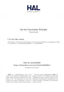


![[hal-00122781, v1] Statistical Matrix Representation of](https://m.moam.info/img/260x300/hal-00122781-v1-statistical-matrix-representation-_5c1b086c097c476f668b4794.jpg)

![[hal-00122781, v1] Statistical Matrix Representation of](https://m.moam.info/img/260x300/hal-00122781-v1-statistical-matrix-representation-_5c1a25d6097c47a0628b4772.jpg)


