Sorting on OTIS-Networks Ehsan Akhgari1, Alireza Ziai1, Mohammad Ghodsi2, 1 Computer Engineering Department, Sharif University of Technology, Tehran, Iran Computer Engineering Department, Sharif University of Technology, Tehran, Iran; School of Computer Science, Institute for Studies in Theoretical Physics and Mathematics, Tehran, Iran {akhgari, ziai}@ce.sharif.edu,
[email protected] 1
2
Abstract. Because of their various desirable properties, OTIS networks are subject to active research in the field of parallel processing. In this paper, the OTIS network architecture is presented, emphasizing two important varieties, the OTIS-mesh and the OTIS-hypercube. Next, a randomized sorting algorithm presented in the literature for OTIS-mesh structures will be reviewed. Finally, a discussion of sorting on OTIS-hypercubes will be offered, and a suggested algorithm for sorting on these networks, with an MPI implementation will be introduced. Keywords: OTIS Network, OTIS-Mesh, OTIS-Hypercube, Sort algorithms
1 Introduction Optical interconnection overcomes the known problems of electrical interconnection, such as the communication bottlenecks in high bit rates and the limitations in case of long distances. Hence, hybrid architectures using both optical and electrical communication links such as the “OTIS 2 Network” are under active research. OTIS is an optoelectronic interconnected network developed for parallel processing systems. The main idea in OTIS Networks is using optical links alongside with electronic links. This idea was first introduced in 2[2]. In OTIS, processors are partitioned into groups (clusters). Intra-group connections are electronic, and the Intergroup connections are optical. For more information on OTIS networks, refer to [4]. The groups inside an OTIS network can be of any of the various parallel processing architectures, including meshes and hypercubes. The resulting architecture will be named based on the underlying group architecture – for example, OTIS-mesh and OTIS-hypercube are OTIS networks resulting from connecting mesh and hypercube structures, respectively. A comparison of the properties of OTIS-mesh and OTIShypercube architectures has been presented in [3].
1 2
This author's work was in part supported by a grant from IPM (N. CS2386-2-01.) Optical Transpose Interconnection System
2 OTIS Network Structure The Intra-group connections (electronic connections) in OTIS networks vary based on the architecture selected for the groups, but the inter-group connections (optical connections) are always formed in a well-known fashion. Suppose that each node is assigned a label in form of ( g , p ) , where g is the group number, and p is the node number in each group. For all i and j , where i ≠ j , the node (i, j ) is connected to the node ( j , i ) using an optic link.
3 Sorting on OTIS-Hypercube Networks An N 2 node OTIS-hypercube is built using N clusters, each being a lg N -cube. The hypercube nodes in each cluster are linked together by electronic links. Following the same convention as the OTIS-Mesh network for numbering the nodes, each node will be assigned a number in form of ( g , p ) , where g is the group number, and p is the node number in each cluster. Using this naming convention, every ( p, g ) node in the network is connected to the ( p, g ) node by means of an optic link. A sample OTIS-hypercube structure appears in Fig. 1. This structure consists of eight 3-cube clusters, as well as the optical links between them. We will proceed to show that an N 2 node OTIS-hypercube has less hardware cost than an N 2 node hypercube. An N 2 node hypercube has N 2 lg N edges, which are all electronic. A similar N 2 node OTIS-hypercube network, on the other hand, consists of N hypercubes, each with ½ N of ½ N
2
(lg N )
(lg N ) edges, which makes a total
(
) pairs in the i ≠ j . Therefore, there are ½ (N − N )
electronic edges. In addition, there are ½ N − N 2
2
form of (i, j ) where 0 ≤ i, j < N and optic edges as well in the OTIS-hypercube network. Therefore, the total number of
( (lg N ) + (N )− N ) .
edges in an N 2 OTIS-hypercube is ½ N
2
2
Fig. 1. A 64-node OTIS-hypercube network, where electronic and optic links are shown using black and blue links, respectively
In order for an N 2 node OTIS-hypercube network to have less edges than an N 2 node hypercube, the following inequality must hold.
(
)
( )
2 N 2 (lg N ) > N 2 (lg N ) + N 2 − N .
(
(1)
)
Eq. 1 can be rewritten in form of N lg N > N − 1 , which holds for each N > 1 . Because the special case N = 1 has only a single processor, and cannot be utilized for any parallel computations, this special case can be ignored. Therefore, we have shown than an N 2 node hypercube has more edges than an N 2 node OTIS-
(
)
hypercube for all practically interesting networks. Furthermore, ½ N − N of the edges of such an OTIS-hypercube network are optical. So, one can safely conclude that the OTIS-hypercube network is less costly than a hypercube network with the same number of nodes. Such a comparison only applies where one of the two networks can be simulated using the other one with a small slowdown. The following theorem establishes that an 2
N 2 node OTIS-hypercube network can actually simulate an N 2 node hypercube. Theorem 1. An N 2 -node OTIS-Hypercube network can simulate an N 2 -node hypercube with a slowdown factor of at most 3. The proof of this theorem appears in 5[5]. The proof is explained informally here as well, because it is used in construction of the sorting algorithms on OTIShypercube networks. Suppose the node ( g , p ) in the OTIS-hypercube is labeled in form of ( g1 L g n p1 L pn ) , where g1 L g n is the binary representation of g ,
p1 L pn is the binary representation of p and n = lg N .
For an OTIS-hypercube to be equivalent to a hypercube, every node in the network must be connected to all nodes which differs from it in exactly one bit position. If the difference bit position is in the lower half (i.e., in p1 L pn ) there is a
direct electronic link between the nodes, because both are located in the same cluster. If the difference bit position is in the upper half, the link can be simulated in at most 3 steps. The first step is using an optic link to move to the node ( p1 L p n g1 L g n ) (the g and p parts of the label are swapped.) After this step, the difference bit lies in the lower half of the label, so the transform can be made locally in the cluster. In the third step, another optic link is traversed to restore the order of g and p in the label. This simulation can happen in 2 steps for the special cases where one of the source or destination addresses is in form of (i, i ) . If the source address is in that form, the first step of the above simulation is unnecessary (and not possible, since nodes with (i, i ) addresses do not have any optic adjacent edges.) Likewise, if the destination address is in that form, the last step of the simulation would be redundant. From Theorem 1, it can be concluded that any hypercube algorithm can be simulated on an OTIS-hypercube network with the constant slowdown of at most 3 (thus, asymptotically equivalent). This includes sorting algorithms on hypercubes as well. Therefore, these algorithms can also be implemented on OTIS-hypercubes, by substituting data movements along the higher dimension half of hypercube nodes with the 3-step simulation laid out above. We will proceed to explain how one sample hypercube sorting algorithm can be adapted to OTIS-hypercube networks. The chosen algorithm is the Odd Even Merge Sort on a hypercube 1[1]. This algorithm works by recursively merging larger and larger sorted lists. In particular, to sort N items, it begins with splitting the items into N sublists of length 1 . Then, pairs of unit-length lists are merged into N/2 sublists of length 2 . The same process goes on so that in the last step of the recursion, 2 sublists of length N/2 are merged to form the final sorted sequence. The running 2
time is O (lg N ) , which doesn't change for the OTIS-hypercube adapted algorithm. 2
The total number of steps in the original algorithm is lg N + lg N . The interesting part of the algorithm, as described in 1[1] is the merging part. The implementation of merging is described on a butterfly network. On a butterfly network, the merging step of the algorithm consists of two passes. During each step of the first pass, the location of the data items in the upper half of the butterfly does not change (the straight edges are used), while the data in the lower half moves towards the cross edges. The last step of the first pass is exceptional in that all of the straight edges are used (even in the lower half). The first pass effectively reverses the order of data items in the lower half. During the second pass, the data flows back in the butterfly network. At each step, if the adjacent pairs are out of order, they are switched using the cross edges, otherwise they are simply moved using the straight edges. The merge step of the algorithm takes 2 lg N steps. Since this algorithm is normal, it can be run in the same running time on a hypercube. To simulate it on an OTIS-hypercube network, the following points must be considered. • The last step of the first pass has no effect on a hypercube (it simply leaves the position of all of the hypercube edges unchanged). Therefore, it can be omitted in the OTIS-hypercube simulation.
• The first pass of the algorithm consists of lg N − 1 steps. The first ½ lg N steps occur on the electronic edges, and therefore can be simulated with no slowdown. Each of the next ½ lg N − 1 steps occur in 3 steps in an OTIS-hypercube network. Altogether, the first pass would take 2 lg N − 3 steps. • The second pass consists of lg N steps. The first ½ lg N steps can each be simulated in 3 steps, and the next ½ lg N can be directly simulated on an OTIS-hypercube using the electronic links. Therefore, the second pass would take 2 lg N steps. Therefore, the total running time of the merge step would be equal to 4 lg N − 3 . So the total time for sorting N numbers will be
(4 lg 2 − 3) + L + (4 lg N − 3) = 2 lg2 N − lg N .
(2)
2
The total number of steps in the original algorithm is lg N + lg N . The simulated 2
algorithm, as previously noted, has the same asymptotic running time ( O (lg N ) ). 2
Specifically, the simulated algorithm takes at most lg N − 2 lg N more steps to complete than the original algorithm.
4 Conclusion This paper reviewed the important related work in the field of sorting algorithms for OTIS networks, and outlined one randomized sorting algorithm on OTIS-mesh architectures. In addition, a new sorting algorithm for OTIS-hypercube structures was suggested.
References 1. 2. 3.
4. 5.
Leighton, F.T.: Introduction to Parallel Algorithms and Architectures: Arrays - Trees - Hypercubes. Morgan Kaufmann, 1992. Marsden, G., Marchand, P., Harvey P., Esener S.: Optical transpose interconnection system architectures. Optics Letters. 18(13). 1083—1085 (1993) Hashemi Najaf-abadi, H. Sarbazi-Azad H.: An empirical comparison of OTIS-mesh and OTIS-hypercube multicomputer systems under deterministic routing. In: 19th IEEE International Parallel and Distributed Processing Symposium, p. 262a. IEEE Press, New York (2005) Pijitrojana, W.: Optical transpose interconnection system architectures. 2003. Francis Zane, Philippe Marchand, Ramamohan Paturi, and Sadik Esener, "Scalable network architectures using the optical transpose interconnection system (OTIS)," Journal of Parallel and Distributed Computing, 60(5):521–538, 2000.