Source Constrained Clustering - Carnegie Mellon University

Source Constrained Clustering Ekaterina Taralova Fernando De la Torre Martial Hebert Carnegie Mellon University {etaralova,ftorre,hebert}@cs.cmu.edu

Abstract We consider the problem of quantizing data generated from disparate sources, e.g. subjects performing actions with different styles, movies with particular genre bias, various conditions in which images of objects are taken, etc. These are scenarios where unsupervised clustering produces inadequate codebooks because algorithms like K-means tend to cluster samples based on data biases (e.g. cluster subjects), rather than cluster similar samples across sources (e.g. cluster actions). We propose a new quantization technique, Source Constrained Clustering (SCC), which extends the K-means algorithm by enforcing clusters to group samples from multiple sources. We evaluate the method in the context of activity recognition from videos in an unconstrained environment. Experiments on several tasks and features show that using source information improves classification performance.

1. Introduction We explore the problem of generating a codebook by clustering features from data with large within-class variability. In particular, we study the problem of data quantization via K-means in the context of a BoW model, which has demonstrated state of the art performance in a wide range of computer vision tasks [3, 15, 19, 28]. The BoW framework relies heavily on the assumption that the clustering step produces a grouping of the samples which is meaningful for the classification task. However, when data comes from disparate sources the resulting clusters might not be suitable for distinguishing between the desired semantic classes. Example scenarios which use data from disparate sources include: activity recognition tasks where multiple subjects perform actions with varied styles in unconstrained environments; object recognition tasks in which the images come from environments with dissimilar characteristics [22]; data from web sources with different presentation style and bias, etc. It is often the case that data collected in such settings exhibits a large within-class variability for a range of semantic

Subject A

Subject B

Video 1A

Video 1B

Video 1A

Video 2A

Video 2B

Video 2A

Video 1B

Video 2B

a)

b)

SCC clusters actions

K-means clusters subjects

1A

1A 1B 2A 2B

1

1A

1B

1B

2A

2A

2B 2

BoW quantization, K-means

0

distances between histograms

c)

1A 1B 2A 2B

1

2B 2

0

distances between histograms

d)

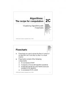
Figure 1. We want to cluster actions performed by different subjects (a). In a BoW framework with K-means, a quick look at the discretized videos (b) reveals clustering of subjects, which is due to the distinctive styles of execution. SCC uses source information and clusters actions, as seen from the χ2 distances between the discretized videos (c) - 1A is closer to 1B, as desired, while with K-means (d) video 1A is closer to 2A (same subject).

categories. This presents a challenge when learning codebooks via unsupervised clustering algorithms, which tend to group samples from the same source, rather than cluster samples from the same semantic class. For example, in Figure 1, features from four video segments are discretized according to a codebook learned via K-means. Due to the different execution styles, the discretized samples from the same source are closer to each other, than to the sample in the same action class. This makes the codebook less suitable for distinguishing between the two action classes. This paper proposes a quantization technique which accounts for the problem of source clustering. We evaluate the method in the context of activity recognition of subjects performing actions in an unconstrained environment.

In addition to a synthetic data set example, we present results on two realistic data sets. First, we analyze the Hollywood 2 data set [13], comprised of 69 different movies with 12 manually labeled action classes. We consider each movie as a source that generates examples in a particular, often unique, style, which is due to producer and genre bias. For example, “driving” could be a clip of a car moving on a street, or a person behind the wheel. In the second data set, the CMU Multimodal database [4], multiple subjects were asked to prepare different recipes. The data set contains tremendous variability within action classes, and even simple tasks such as cracking an egg or opening a package are performed in a multitude of ways and styles. To address the large variability across sources, we propose Source Constrained Clustering (SCC), which imposes the constraint that each cluster includes samples from several sources. We ground this idea in the widely used setting of learning a codebook for a bag-of-words (BoW) model. This framework represents an image or video sequence as an orderless collection of local features. The standard algorithm proceeds by clustering all the training features, discretizing the original data using the learned cluster centers, and finally training a model for classification of new examples. The usual K-means clustering step in a BoW framework is replaced by a new optimization step which incorporates these source constraints. The new constraints require source information for each training data sample, which is generally readily available, or otherwise easy to annotate (e.g., subject id or movie id, etc.). Our hypothesis is that 1) we can incorporate source constraints in a K-means formulation; 2) source information produces better quantization of the data according to semantic classes. We evaluate this hypothesis across three data sets and three types of features and show improvement in classification performance when source information is used to learn a codebook in a BoW setting.

2. Prior work One example of prior work on activity recognition where data comes from disparate sources is the Hollywood 2 data set [13]. Video clips in the same action class but extracted from different movies vary greatly in their visual characteristics. Marszalek et al. [13] report classification results of average precision 0.326 using a BoW framework and STIP features, clearly showing the difficulty of the problem. The same approach applied to action classification from YouTube videos of sport events shows that BoW approaches on real world data sets need further improvement [16]. Similarly, prior work on clustering features extracted from video sequences from the CMU Multimodal Database [4] shows that several algorithms cluster samples from the same subjects, rather than discriminate samples across action classes. This type of data sets (and simi-

larly [21, 14]) presents a challenge to standard codebook learning algorithms because subjects perform the same actions in very different ways (e.g. cracking an egg using a fork, the rim of a bowl, finger, or on the counter surface). The bias of data from such unconstrained environments complicates the creation of robust codebooks, because the learned clusters represent styles, rather than contain representative samples from multiple sources. The solution we propose is an extension of the Kmeans [12] algorithm – one of the most widely used techniques for clustering and learning codebooks, due to its simplicity and good performance. This work is inspired by the constrained K-means clustering method proposed by Bradley et al. [2], in which new constraints ensure that each cluster contains a minimum number of data samples. Our algorithm differs from this work by imposing a different set of constraints – each cluster should contain data from multiple sources. Among many other K-means extensions, the work of Wagstaff et al. [24] is closely related to ours. The authors extend K-means with must-link and cannotlink constraints specified directly on the features using domain knowledge. This algorithm and its many extensions, like soft-constrained clustering [11], have shown excellent results. However, these methods are not suitable in scenarios with interest samples or aggregate features statistics, where we do not have knowledge of how to constrain individual data samples. This paper builds on existing work on discriminative clustering [5, 7, 1, 26]. Generative methods for clustering such as K-means and spectral clustering do not provide a feature selection or feature weighting mechanism to remove irrelevant features for clustering. In our scenario, we are interested in weighting the features such that each cluster contains multiple disparate sources. Discriminative clustering algorithms combine distance metric learning [18, 25] with clustering algorithms. Typically, discriminative clustering algorithms compute a low dimensional projection that also encourages cluster separability. Unlike previous discriminative clustering algorithms [5, 7, 1, 26] which are unsupervised, this paper proposes to weakly guide clustering and metric learning using source information.

3. Background 3.1. Regular clustering (RC): K -means Consider the problem of clustering N data samples into K clusters. Let D be a D × N real matrix of samples where D is the data dimension and N is the number of samples. Kmeans clustering splits a set of N samples into K groups by minimizing the within-cluster variation. That is, K-means finds a grouping of the data that is a local optimum of the following energy function [27, 6, 5]:

minimize G,M kD − MGT k2F subject to:

K X

gic = 1, ∀i ∈ [1, N ]

(1a) (1b)

and thus the objective in (2a) becomes:

tr BT Sw B ∝ tr BT (D − MGT )(D − MGT )T B (4a) = kD − MGT k2B ,

(4b)

c=1

G : Binary

(1c)

where G is a N × K binary indicator matrix with elements gic specifying if point i belongs to cluster c, and M is the D × K matrix of data means (see notation1 ). The K-means algorithm performs coordinate descent in (1a). Given an initial value for M, the algorithm iterates between optimizing for G and recomputing M, until the change in objective is small, or a maximum number of iterations is reached. The constraint (1b) enforces that each data point belongs to only one cluster.

which is the K-means objective from (1a), weighted by a projection matrix B. We optimize the following error function, which combines metric learning (dimensionality reduction) and K-means clustering, and which we term RC LDA: minimize G,M,B kD − MGT k2B subject to:

where B is a D × (K − 1) projection matrix, and the covariance matrices are defined as: Sw =

k 1 XX (di − mc )(di − mc )T N − 1 c=1

St =

1 N −1

(di − m)(di − m)T

(3b)

i=1

4. Regular Clustering (RC) with LDA Following existing work in discriminative clustering [5, 7, 1, 26], we formulate an energy function for joint clustering and metric learning with dimensionality reduction. A key observation is that we can re-write Sw in terms of the cluster assignment matrix G:

1 Bold


tr BT St B ≥ 1

(5c)

G : Binary

(5d)

We perform coordinate descent and alternate between clustering with K-means in the projected space and computing LDA. That is, we iterate between: 1) for a fixed B, solve the standard K-means problem specified in (1); 2) for fixed G and M, solve for the projection matrix, B, via the generalized eigenvalue problem St B = Sw BΛ. We stop when the change in objective is small or until a maximum number of iterations has been reached. Unlike [7], we use the total covariance matrix St , which is more suitable for expressing the source constraints in the next section. We use K-means, which differs from the work of [5], who use a continuous formulation to estimate G.

5. Source constrained clustering (SCC)

where the data mean is denoted by m and mc is the mean for cluster c.

Sw =

(5b)

(3a)

di ∈c

N X

gic = 1, ∀i ∈ [1, N ]

(5a)

c=1

3.2. Linear Discriminant Analysis (LDA) LDA is a supervised algorithm which finds a projection of the data onto a subspace where the distance between clusters is maximized, while the distance within each cluster c ∈ [1, K], is minimized. The formulation we use is [8]:
minimize B tr BT Sw B (2a)
T subject to: tr B St B ≥ 1 (2b)

K X

1 (D − MGT )(D − MGT )T , N −1

capital letters denote a matrix X, bold lower-case letters a column vector x. xi represents the ith column of the matrix X and xij denotes the scalar in the ith row and j th column. IN is the N × N identity matrix, 1N is a column vector of ones. kXk2F = tr(XT X) = tr(XXT ) is the Frobenious norm of X, and kXk2B = tr(XBBT XT ). The Kronecker product Am×n ⊗ Bp×q produces an mp × nq block matrix.

5.1. Overview When quantizing data from disparate sources, we want to discover clusters which 1) group similar samples and 2) are representative of the sources. For example, in activity recognition, K-means might cluster the particular styles of subjects performing actions. However, we seek a discretization that generalizes the styles, i.e. clusters which are representative of the subjects. While it is impossible to know the optimal number of sources that should be represented in each cluster, SCC approximates this problem by constraining that each cluster contains a minimum number of sources. Formally, we consider the problem of clustering N samples from R sources into K clusters, such that each cluster contains data from at least a fixed number of sources, h. For each data point i ∈ [1, N ], we are given the source id, s ∈ [1, R], which generated this point. We can add source constraints to K-means by counting the number of sources represented in each cluster. First, we re-write the RC LDA problem (5) in a form that will allow us to write a linear integer program (LIP) with

constraints that require each cluster to represent a minimum number of sources. Then, we show the derivation of the matrices used in the source constraints, and we present the final SCC optimization problem.

5.2. RC LDA reformulation We denote by vec(G) the column vector produced by concatenating the columns of the matrix G, so that the first N entries, g11 . . . gN 1 , contain a 1 for samples in cluster 1, the next N entries, g12 . . . gN 2 , contain a 1 for samples in cluster 2, and so forth:  T vec(G) = g11 . . . gN 1 . . . g1K . . . gN K N K . (6) The constraints in (5b) which ensure that a point belongs to only one cluster can be expressed as: Uvec(G) = 1N ,

(7)

where UN ×N K = 1TN ⊗ IN . The objective function (5a) can be expressed using vec(G) and a column vector fN K which contains the squared distances from each data point to each cluster center:  T (d1 − m1 )T BBT (d1 − m1 )    ...    (dN − m1 )T BBT (dN − m1 )    ..  f T vec(G) =  vec(G).   .    T T  (d1 − mk ) BB (d1 − mk )    ... (dN − mk )T BBT (dN − mk ) NK



(8) The RC LDA optimization problem (5) can be written as: minimize G,M,B f T vec(G) subject to: Uvec(G) = 1N
tr BT St B ≥ 1 G : Binary

(9a) (9b) (9c)

-

cluster assignments for each point (binary) hard cluster assignment K-means (binary) source assignments per cluster (binary) sum unique sources in a cluster (binary) source assignments for each point (binary) select sources represented in each cluster (binary) select total number of samples in a cluster (binary)

Table 1. Matrices used in the SCC integer program formulation.

ensures that xcs is set to 0 if source s does not have any points in cluster c. LIP formulation. We now write the source constraints in matrix form for all clusters. Let X be the K × R binary matrix whose entries are xcs . Then (10) can be written as:
Vvec(X) = 1TR ⊗ IK vec(X) ≥ h1K .

(12)

We can write (11) for all clusters and all sources as: vec(X) ≤ Pvec(G),

(13)

where the RK × N K binary matrix P selects the samples each source has in the cluster specified by G. To construct P, we represent the source information in a N × R binary matrix Q, with elements qis = 1 if point i comes from source s, and 0 otherwise. To get the number of samples source 1 has in each cluster, take q1 , the first column of Q, and duplicate it K times: e 1 vec(G) = (IK ⊗ qT )vec(G), ws = Q 1

(14)

so that the vector ws of length K contains the number of e 1 is a K × N K binary samples s has in each cluster, and Q matrix. Repeating for each source, the per cluster source information matrix P is given by:

(9d) 

5.3. Source constraints Sketch. First, we describe the source constraints for a cluster c, then we construct the matrices used by the final linear integer program (see Table 1). We enforce each cluster c to have samples from at least h sources by constructing the sum over all sources in the cluster and thresholding it by h. If xcs is a binary variable equal to 1 when source s has at least one data point in cluster c, we can express this as: R X

GN ×K UN ×N K XK×R VR×K QN ×R PRK×N K RRK×N K

 e1 Q   P =  ...  eR Q

.

RK×N K

The optimization problem (9) with source constraints is: minimize G,M,B,X f T vec(G) subject to: Uvec(G) = 1N vec(X) − Pvec(G) ≤ 0

xcs ≥ h.

(10)

s=1

Let wcs ≥ 0 be the number of samples source s has in cluster c, as assigned by G. Since xcs ∈ {0, 1}, the inequality xcs : Binary and xcs ≤ wcs

(11)

(15)

(16a) (16b) (16c)

Vvec(X) ≥ h1K
tr BT St B ≥ 1

(16d)

G, X : Binary

(16f)

(16e)

5.4. Regularization Constraints (16c) and (16d) ensure that each cluster contains samples from at least h sources. However, this does not guarantee that the sources contribute a meaningful number of samples in participating clusters. Indeed, an undesirable solution would be to assign to cluster c some samples from source s = 1, and only one data sample from each of the remaining s = 2 . . . h sources. To account for this, we add a regularizing constraint to ensure each source contributes a non-trivial amount in every participating cluster. Sketch. Let tc be the total number of samples in cluster c and assume every cluster has at least h sources. We approximate the fraction of samples sources should have in samples of tc . We coneach cluster by a fraction of h+R 2 strain wcs , the number of samples s has in c, to be within ˜ s samples of this quantity: θn ˜ s, wsc ≥ γtc − θn

(17)

(18)

where the right-hand side is θs if s has at least one point in c (xcs = 1), or it evaluates to N otherwise. In the latter case, the constraint is trivially satisfied, since xcs = 0 implies wsc = 0, and it is always the case that γtc ≤ N . LIP formulation. The total number of samples in c = 1 are obtained by summing up the first N entries of vec(G): t1 = [1TN 0TN . . . 0TN ]vec(G).

(20)

(21)

We re-write (18) as: γtc − wsc + (N − θs )xcs ≤ N.

The final SCC optimization problem is: minimize G,M,X,B f T vec(G) subject to: Uvec(G) = 1N vec(X) − Pvec(G) ≤ 0 Vvec(X) ≥ h1K

(24a) (24b) (24c) (24d)

(γR − P)vec(G) + (N 1TRK − θ T )vec(X) ≤ N 1RK (24e)
T (24f) tr B St B ≥ 1 (24g)

We approximately solve (24) as in [5, 7] by initializing M to K samples at random, setting B = I, and iterating between: 1) solving for G and M in the standard K-means setting, with B fixed; and 2) solve for B, using G and M found in the previous step (see Algorithm 1). To solve the LIP problem, we use the ILOG CPLEX [9] software. Algorithm 1 SCC(D, M, h) for t = 0... do // iterative clustering and metric learning for s = 0... do // iterative SCC fs ← ComputeObjective(Dt , Ms ) (G∗s+1 , X∗s+1 ) = SolveLIP(fs , h) // Eq. (24) Ms+1 ← ComputeMeans(Dt , G∗s+1 ) end for Mt+1 ← Ms , Gt+1 ← G∗s Bt ← LDA(Gt+1 , Mt+1 ) // metric learning Dt+1 ← BTt Dt ; Btotal ← BTt Btotal end for return Gt , Btotal

6. Experiments

and for all sources we construct the binary selector matrix: e RRK×N K = 1R ⊗ R.

5.5. SCC algorithm

(19)

For all clusters we can write: e K×N K = (IK ⊗ 1T ), R N

γRvec(G) − Pvec(G) + (N 1TRK − θ T )vec(X) ≤ N 1RK , (23) where θ = 1K ⊗ [θ1 . . . θR ]T , a vector of length RK.

G, X : Binary

2 where γ = h+R , and ns is the total number of training ˜ s samples samples generated by source s. The slack of θn account for the case where the number of training samples per source can differ greatly, and we cannot expect sources to contribute the same number of samples. First, we set θ˜ = 0, which approximates a uniform source distribution. If the problem is infeasible, we relax it and try a range of thresholds that take into account the number of samples per source. We vary θ˜ from 0.05 to 0.4 in increments of 0.05, ˜ s . Furthermore, (17) should hold only and define θs = θn if the solution assigns non-zero number of samples from s to c, i.e. when xcs = 1, otherwise the constraint should be inactive:

γtc − wsc ≤ θs xcs + N (1 − xcs ),

Using P and X defined in the previous section, constraint (22) for all clusters and all sources becomes:

(22)

We show that using source information when data comes from disparate sources improves classification in a BoW codebook task. Furthermore, we confirm that the improvement in performance is correlated with the source variance. To show that the approach can be applied to a broad class of vision tasks, we perform experiments on three data sets and three types of features in BoW classification tasks. First, we illustrate SCC on a simple synthetic data set, then we compare to previously reported results on the Hollywood 2 action data set [13], and finally we report results on action classification on the CMU-MMAC data set [4].

Class 1 Class 2

Feature samples from sequence 1

Source A

Feature samples from sequence 2

Cluster 1 Cluster 2 Cluster 3 Cluster 4 Cluster 5 X Means

Cluster 1 Cluster 2 Cluster 3 Cluster 4 Cluster 5 X Means

Source B

Source C

Source D

x=5

y = 10

Sequence 1, quantized

Cluster ids

1 2 3 4 5

1 2 3 4 5

1 2 3 4 5

1 2 3 4 5

1 2 3 4 5

1 2 3 4 5

1 2 3 4 5

1 2 3 4 5

1 2 3 4 5 Class 1

1 2 3 4 5 Class 2

Source E

a) Input

b) K-means clusters

c) SCC clusters

d) SCC quantization

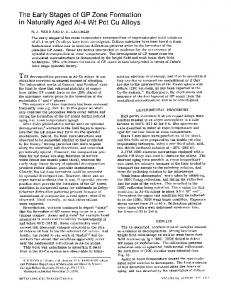
Figure 2. Synthetic data where samples generated by the same source are closer than the samples in the same class (see Section 6.1). K-means groups sources (b), resulting in a non-discriminative feature quantization. Our algorithm, SCC, with h = 3, produces a more meaningful clustering, as shown in (c) with rough cluster outlines. The quantized data is clearly separated into the two classes (d).

Given a data set of action sequences with class labels we follow the standard procedure for codebook creation in BoW frameworks. This includes extracting features (in our case, STIP [10] and GIST [23]); generating disjoint training, validation and testing sets; clustering training features to learn a codebook; discretizing the features using the learned cluster centers; and training a discriminative classifier. We train a one-versus-all χ2 SVM classifier [17] and report average precision (AP) as in [13]. We evaluate three codebook creation schemes: RC Eq. (1), RC LDA Eq. (9), and SCC Eq. (24) in two unsupervised tasks and two supervised tasks. The former setting is the standard codebook creation scheme which clusters all the features in an unsupervised way. In the latter setting we use the training labels to cluster samples within each class, creating one codebook per class. This is useful in practice when large amounts of data limit the size of the optimization problem that can be solved efficiently. We experiment with K = 30, 40, 60, 100 clusters. First, we validate the method works even for a fixed value of the parameter h = 5 for all experiments - a reasonable choice, since h = 0 is RC, while h = R would imply all sources should participate in all clusters, which is unrealistic in these data sets. Second, we confirm SCC is not sensitive to the choice of h by setting h = 2, 3, 5, 7, 10 and noting a maximum change in overall AP of around 2%. For comparison, we also report results with varying values of h per class, based on manual inspection of the per-class performance. A complete validation system for discovering the optimal h for each class would require a large amount of validation data, currently unavailable for these data sets.

6.1. Synthetic experiment We build a synthetic data set of 5 sources generating a sequence in each of two classes, 1 and 2. The sequences are bags of ten 2D samples. The first component of the features, x, is correlated with the class id, while the second, y, is correlated with the source id. The samples are drawn from Gaussian distributions with parameters chosen to simulate disparate sources. For every source yi , the distance between the samples in the bag from class 1 and the bag from class 2 is smaller than the distance to the correct class bag from other sources (∆x < ∆y), as shown in Figure 2. Figure 2 shows one representative clustering for K = 5. RC clusters the samples from the same source – the discretized sequences from class 1 are nearly identical to the discretized sequences from class 2, making it impossible to train a classifier to distinguish the two classes. On the other hand, SCC produces a quantization of the sequences which clearly discriminates the two classes. For ease of visualization, Figure 2 (d) shows the rough boundaries of the SCC clusters in the original feature space (not LDA).

6.2. Hollywood movie data set We use the clean dataset provided by the authors, which contains 1707 action samples divided into a training set (823 sequences) and a disjoint test set (884 sequences). Following [13], we subsample the STIPs at random, retaining 10% of the features for training. To further reduce the computational complexity, we learn a codebook per training action class. As shown in Table 2, we verify that performance of per class codebooks is comparable to published results [13], and thus the method is suitable for compari-

AnswerPhone DriveCar Eat FightPerson GetOutCar HandShake HugPerson Kiss Run SitDown SitUp StandUp Mean AP

Marszalek et al. 0.088 0.749 0.263 0.675 0.090 0.116 0.135 0.496 0.537 0.316 0.072 0.350 0.324

RC 0.103 0.797 0.381 0.564 0.195 0.100 0.188 0.442 0.422 0.331 0.099 0.342 0.330

RC LDA 0.098 0.794 0.465 0.584 0.162 0.112 0.154 0.433 0.494 0.351 0.093 0.360 0.342

SCC h=5 0.112 0.824 0.382 0.620 0.174 0.166 0.195 0.420 0.489 0.372 0.131 0.449 0.361

SCC varied h 0.116 4 0.841 7 0.493 3 0.630 7 0.174 5 0.172 7 0.212 3 0.437 2 0.476 2 0.399 2 0.131 5 0.449 4 0.378

Table 2. Comparison of clustering methods for learning per class codebooks from HoG+HoF features on the Hollywood 2 [13] data set. SCC improves mean AP by 3.1%compared to RC, and 1.9% compared to RC LDA for a fixed h = 5. Class specific value of h gives a further 1.7% increase. As a reference to learning a global codebook, the results from [13] are shown in the left column.

son. Table 2 shows the results with K = 100 for the three clustering algorithms along with the previously published results of Marszalek et al. [13]. We see improvement in performance for 10 out of 12 actions compared to both RC and RC LDA. The classes for which SCC performs better than RC have a larger number of training sources and exhibit stronger source clustering. In these scenarios, using source information helps build more robust codebooks.

6.3. CMU kitchen data set The Carnegie Mellon University Multimodal Activity database (CMU-MMAC) [4] contains multimodal measurements of subjects performing different recipes with no prior instructions. The actions vary greatly in time span, repetitiveness, and manner of execution. From the 35 manually annotated action classes from [20] we merge semantically similar ones ( e.g. “take from cupboard left” and “take from cupboard right” are combined, etc.), and we ignore actions which have a very small number of instances. In total we have 15 classes listed in Table 3. We use the videos from the wearable camera and extract STIP and GIST features from every fifth frame. 14 subjects are used for training and two for testing. We average results over 4 disjoint sets of withheld subjects, chosen at random. 6.3.1

Per class codebook using STIP features

Following the procedure of [13], we subsample the STIPs at random, retaining 20% of the training data for learning a codebook. Again, to allow for more training samples to be used, we cluster samples in each class, learning one codebook and distance metric transformation per class. In Table 3 we report results for h = 5 and K = 40.

crack-egg open-bag fridge-door pour-oil pour-bowl put-obj-lower spray-pam stir-egg read-switch take-fridge take-drawer take-top take-bottom twist-cap walk Mean AP

RC 0.775 0.683 0.891 0.567 0.660 0.397 0.889 1.000 0.863 0.633 0.569 0.891 0.394 0.547 0.966 0.715

STIP RC LDA 0.787 0.640 0.906 0.198 0.685 0.402 0.595 1.000 0.807 0.676 0.503 0.733 0.567 0.560 0.951 0.667

SCC 0.733 0.707 0.922 0.563 0.724 0.386 0.778 1.000 0.844 0.611 0.710 0.872 0.654 0.533 0.969 0.734

RC 0.119 0.296 0.669 0.030 0.302 0.641 0.534 0.071 0.416 0.309 0.705 0.817 0.561 0.091 0.563 0.408

GIST RC LDA 0.125 0.191 0.515 0.050 0.530 0.727 0.493 0.088 0.515 0.283 0.485 0.846 0.502 0.295 0.340 0.398

SCC 0.289 0.240 0.594 0.031 0.528 0.717 0.725 0.207 0.595 0.490 0.736 0.772 0.521 0.206 0.524 0.478

Table 3. Classification performance on the CMU-MMAC [4] data set using STIP and GIST features. Using the source information increases the mean AP by 2.5% for STIPs, and by 7% for GIST, compared to RC.

A quick look at the videos shows large variability in styles for the classes which show improvement, especially for the “taking from drawer” and “taking from bottom cupboard.” On the other hand, for classes with low or no improvement, we observe less style variability. For example, the action “walk” from the counter to the fridge was performed without much variance, and likewise for “stirring egg,” and regular clustering has no problem in classifying such actions nearly perfectly. The 2.5% average increase in AP for this task also shows the benefits of using source information. 6.3.2

Global codebook using GIST features

Prior work on the CMU-MMAC data set reports source clustering when using GIST features [20]. These features encode the style of execution more strongly and we see a more pronounced source clustering problem compared to using STIPs (several of the RC clusters contain samples only from one subject). Our hypothesis is that using source information in this case will have an even stronger impact on performance. Indeed, the results in Table 3 show a 7% improvement in AP when learning a global codebook in an unsupervised manner using features from 11 training subjects, and testing on 5 subjects., with K = 40 and h = 5. There is a clear improvement in performance for 9 out of 15 classes. This additional experiment verifies that the concept of SCC is beneficial across different types of features.

7. Conclusion In this paper we presented SCC – a novel extension of Kmeans for quantization of data generated by diverse sources.

Our experiments show improvement in classification performance across several tasks and features compared to standard K-means in a BoW framework. In future work, SCC can be applied to other interesting scenarios. For example, training object detectors on data with large bias obtained by combining multiple data sets [22]. In addition, SCC can be applied to non-vision data sets, for instance in topic modeling from websites with different writing styles.

8. Acknowledgements This work is based on work supported by the National Science Foundation under Grant No. EEEC-0540865.

References [1] F. Bach and Z. Harchaoui. Diffrac : a discriminative and flexible framework for clustering. In NIPS, 2007. 2, 3 [2] P. S. Bradley, K. P. Bennett, and A. Demiriz. Constrained K-Means Clustering. Technical report, 2000. 2 [3] C. Dance, J. Willamowski, L. Fan, C. Bray, and G. Csurka. Visual categorization with bags of keypoints. In ECCV International Workshop on Statistical Learning in Computer Vision, 2004. 1 [4] F. De la Torre, A. Bargeil, X. Martin, and J. Hodgins. Guide to the cmu multimodal activity (cmu-mmac) database. http://kitchen.cs.cmu.edu/. In Tech. report, Robotics Institute, CMU, 2008. 2, 5, 7 [5] F. De la Torre and T. Kanade. Discriminative cluster analysis. In International Conference on Machine Learning, volume 148, pages 241 – 248, New York, NY, USA, June 2006. ACM Press. 2, 3, 5 [6] C. Ding and X. He. K-means clustering via principal component analysis. In International Conference on Machine Learning, volume 1, pages 225–232, 2004. 2 [7] C. Ding and T. Li. Adaptive dimension reduction using discriminant analysis and k-means clustering. In International Conference on Machine Learning, 2007. 2, 3, 5 [8] K. Fukunaga. Introduction to Statistical Pattern Recognition, Second Edition. Academic Press.Boston, MA, 1990. 3 [9] ILOG. IBM ILOG CPLEX optimizer, 2010. http:// www.ilog.com/products/cplex/. 5 [10] I. Laptev and T. Lindeberg. Local descriptors for spatiotemporal recognition. In International Workshop on Spatial Coherence for Visual Motion Analysis, volume 3667, pages 91–103, 2006. 6 [11] M. H. Law, A. Topchy, and A. K. Jain. Clustering with Soft and Group Constraints. Structural, Syntactic, and Statistical Pattern Recognition, pages 662–670, 2004. 2 [12] J. B. MacQueen. Some methods for classification and analysis of multivariate observations. In 5-th Berkeley Symposium on Mathematical Statistics and Probability.Berkeley, University of California Press., pages 1:281–297, 1967. 2 [13] M. Marszalek, I. Laptev, and C. Schmid. Actions in context. In IEEE Conference on Computer Vision & Pattern Recognition, 2009. 2, 5, 6, 7

[14] R. Messing, C. Pal, and H. Kautz. Activity recognition using the velocity histories of tracked keypoints. In Proceedings of the Twelfth IEEE International Conference on Computer Vision, 2009. 2 [15] K. Mikolajczyk, C. Schmid, and A. Zisserman. Human detection based on a probabilistic assembly of robust part detectors. In European Conference on Computer Vision, volume 3021, pages 69–82. Springer Berlin, 2004. 1 [16] J. C. Niebles, C. Chen, and L. Fei-Fei. Modeling temporal structure of decomposable motion segments for activity classification. In Proceedings of the 11th European Conference on Computer vision, pages 392–405. Springer, 2010. 2 [17] B. Scholkopf and A. J. Smola. Learning with Kernels: Support Vector Machines, Regularization, Optimization, and Beyond. MIT Press, Cambridge, MA, USA, 2001. 6 [18] N. Shental, T. Hertz, D. Weinshall, and M. Pavel. Adjustment learning and relevant component analysis. In Proceedings of the 7th European Conference on Computer VisionPart IV, pages 776–792, London, UK, 2002. Springer. 2 [19] J. Sivic, B. Russell, A. Efros, A. Zisserman, and W. Freeman. Discovering objects and their location in images. In 10th IEEE International Conference on Computer Vision, volume 1, pages 370 – 377 Vol. 1, 2005. 1 [20] E. Spriggs, F. De La Torre, and M. Hebert. Temporal segmentation and activity classification from first-person sensing. In CVPR Workshop on Egocentric Vision, pages 17 –24, 2009. 7 [21] M. Tenorth, J. Bandouch, and M. Beetz. The TUM Kitchen Data Set of Everyday Manipulation Activities for Motion Tracking and Action Recognition. In IEEE Int. Workshop on Tracking Humans for the Evaluation of their Motion in Image Sequences (THEMIS), 2009. 2 [22] A. Torralba and A. Efros. Unbiased look at dataset bias’. In Conference on Computer Vision and Pattern Recognition, 2011. 1, 8 [23] A. Torralba and A. Oliva. Statistics of natural image categories. Network: Computation in Neural Systems, 14:391– 412, 2003. 6 [24] K. Wagstaff, C. Cardie, S. Rogers, and S. Schroedl. Constrained K-means Clustering with Background Knowledge. In Proceedings of 18th International Conference on Machine Learning, pages 577–584, 2001. 2 [25] E. P. Xing, A. Y. Ng, M. I. Jordan, and S. Russell. Distance metric learning, with application to clustering with side-information. In Advances in Neural Information Processing Systems 15, volume 15, pages 505–512, 2002. 2 [26] J. Ye, Z. Zhao, and M. Wu. Discriminative k-means for clustering. In Advances in Neural Information Processing Systems, 2007. 2, 3 [27] H. Zha, C. Ding, M. Gu, X. He, and H. Simon. Spectral relaxation for k-means clustering. In Neural Information Processing Systems, pages 1057–1064, 2001. 2 [28] J. Zhang, M. Marszalek, S. Lazebnik, and C. Schmid. Local features and kernels for classification of texture and object categories: A comprehensive study. International Journal of Computer Vision, 73:213–238, June 2007. 1