SOURCE EXTRACTION IN AUDIO VIA BACKGROUND LEARNING YANG WANG AND ZHENGFANG ZHOU
Abstract. Source extraction in audio is an important problem in the study of blind source separation (BSS) with many practical applications. It is a challenging problem when the foreground sources to be extracted are weak compared to the background sources. Traditional techniques often do not work in this setting. In this paper we propose a novel technique for extracting foreground sources. This is achieved by an interval of silence for the foreground sources. Using this silence interval one can learn the background information, allowing the removal or suppression of background sources. Very effective optimization schemes are proposed for the case of two sources and two mixtures.
1. Introduction Blind source separation (BSS) is a major area of research in signal processing with a vast literature, particularly in audio signal processing. It aims to separate source signals from their mixtures without assuming detailed knowledge about the sources and the mixing process. One particular application of BSS in audio is to extract a desired audio source from mixtures involving noise, background or unwanted sources. In many practical applications such as mobile and car phones the background may in fact be stronger, even much stronger sometimes, than the desired signal. This can pose a daunting challenge. The basic setup for BSS in audio has n audio sources S1 (t), . . . , Sn (t) and m mixtures X1 (t), . . . , Xm (t), with the model (1.1)
Xk (t) =
k,i L N X X
ak,i,j Si (t − dk,i,j ),
k = 1, . . . , M
i=1 j=1
where ak,i,j are the mixing coefficients and dk,i,j are the delays from the source i to the recording or sensing device k. The multiple delays are a result of reverberations in the ambient environment. In audio applications these mixtures are recordings made by placing m microphones in various locations. In BSS these coefficients are unknown. With the Key words and phrases. Background audio source removal, blind source separation, convolution, reverberation, audio source cancellation, learning, quadratic programming. The first author is supported in part by the National Science Foundation grant DMS-0813750. 1
2
YANG WANG AND ZHENGFANG ZHOU
presence of reverberations we often refer to the mixtures Xk in (1.1) as convolutive mixtures. A more concise way to formulate the model (1.1) is (1.2)
Xk =
L X
Ak,i ∗ Si ,
k = 1, . . . , M
i=1
where ∗ denotes convolution and Nk,i
(1.3)
Ak,i (t) =
X
ak,i,j δ(t − dk,i,j )
j=1
are the convolutive kernels that represent the mixing of both the direct signals and their reverberations. BSS techniques aim to compute these convolutive kernels Ak,i . The bulk of the studies in BSS employ the independent component analysis (ICA) model, where the source signals Sk , modeled as random variables, are assumed to be independent, see the reviews [3, 5] and the references therein for more details. Under this model, many techniques such as Joint Approximate Diagonalization Eigenmatrices (JADE) [2] and Information Maximization (Infomax) [1, 4], as well as their refinements, have been developed. An alternative technique is the Degenerative Unmixing and Estimation Technique (DUET), which uses time-frequency separations to achieve BSS and has the advantage that it can work in the degenerative case M < L, see e.g. [6, 9]. All these techniques have their respective strengths and weaknesses, which are well documented in the literature so we will not go into details here. While these techniques can yield good results in BSS, they all have certain limitations that pose challenges for many source extraction and background removal applications. One of the major challenges is that they do not work well for source extraction if the desired source signals are very weak in comparison to the unwanted sources in the mixtures. Computational cost can be another issue for many practical applications such as mobile and car phone where removing background sources must be done in real time. The batch processing techniques used by many of the ICA techniques do not adapt well to dynamic real-time processing. In source extraction problems we are given mixtures that contain several sources. We shall call those sources that we wish to extract foreground sources and those we wish to remove background sources. In this paper we propose a novel method for removing or suppressing background sources in audio mixtures, thus allowing us to bring out or enhance the foreground sources. The method requires that the foreground sources have an interval of
SOURCE EXTRACTION IN AUDIO VIA BACKGROUND LEARNING
3
silence, i.e. during an interval of time the foreground sources are inactive. This interval does not need to be long. For audio signals often less than 1 second is sufficient but optimal result is achieved around 2 seconds. In most relevant applications such as mobile or car phone this requirement is not an issue. The main idea is that the convolution kernels Ak,i in the model (1.2), although they depend on numerous factors such as building material and shape, are determined entirely by the ambient environment as long as the background sources remain stationary relative to the ambient environment. The interval of silence allows us to learn the ambient environment and estimate the convolutive kernels, from which background sources can be removed by cancelation.
2. Background Cancellation via Learning In practice the time is discretized through sampling. It is convenient to write the convolutive mixtures in the discrete form: (2.1)
Xk (t) =
L X N X
ak,i,j Si (t − j),
k = 1, . . . , M,
i=1 j=0
where t ∈ Z and T0 ≤ t < T1 . The integer N denotes the maximal delay in the mixture, which depends on the ambient environment and the sampling rate. We shall view a signal as an element in l∞ (Z). We shall adopt some standard notations here: For each u =∈ l∞ (Z) we use u(j) to denote its j-th entry and supp (u) its support, i.e. the set of indices of its nonzero entries. For and u, X ∈ l∞ (Z) where u is finitely supported the convolution u ∗ X ∈ l∞ (Z) is defined by u ∗ X(t) =
X
u(j)X(t − j).
j∈Z
Again we may rewrite the model (2.1) simply as (2.2)
Xk =
n−1 X
uk,i ∗ Si ,
k = 1, . . . , m
i=1
where uk,i ∈ l∞ (Z) is supported on [0, N ] with ak,i,j as its j-th element. Suppose that the sources S1 , . . . , SJ are the background sources we wish to remove and SJ+1 , . . . , SL are the foreground sources we wish to extract from the mixtures Xk , 1 ≤ k ≤
4
YANG WANG AND ZHENGFANG ZHOU
M . For any finitely supported bk ∈ l∞ (Z) we have bk ∗ Xk =
L X
bk ∗ uk,i ∗ Si .
i=1
It follows from (2.2) that (2.3)
M X
bk ∗ Xk =
(2.4)
PM
k=1 bk
M X
bk ∗ uk,i ∗ Si .
∗ uki = 0 for 1 ≤ i ≤ J, then L ³X M X
bk ∗ Xk =
k=1
´
i=1 k=1
k=1
If we can find bk such that
L ³X M X
´ bk ∗ uk,i ∗ Si .
i=J+1 k=1
The unwanted background sources are now removed, leading to the extraction of foreground sources. We shall call those bk cancellation kernels. Note that although using this technique the foreground sources are now subject to further convolutions, in general it does not degrade the foreground signals as long as the maximum delay N is not too large and the cancellation kernels not too dense. A human auditory system does not appear to be very sensitive to moderate convolutions. Furthermore, moderate convolutions do not introduce any artifacts to the extract source signals. This is a definite advantage over ICA based techniques or DUET. One question is whether the cancellation kernels exist in general. We shall show that they do in all non-degenerative setting M > J. For each X ∈ l∞ (Z) we associate it with a symbolic Fourier series b X(ξ) =
X
X(n)e−n (ξ),
n∈Z
where eb (ξ) := e2πibξ . We shall refer to this series simply as the Fourier transform of X. b (ξ) is a trigonometric polynomial. It is well Note that if u ∈ l∞ (Z) has finite support than u b Furthermore, τd b \ b X. known that u ∗X = u q X = eq (ξ)X(ξ) where τq X denotes X shifted to the right by q positions. Proposition 2.1. Let uk,i ∈ l∞ (Z) for 1 ≤ k ≤ M and 1 ≤ i ≤ J have finite support. Suppose that M > J. Then there exist finitely supported cancellation kernels b1 , . . . , bM ∈ l∞ (Z) not all zero such that M X k=1
bk ∗ uk,i = 0,
i = 1, . . . , J.
SOURCE EXTRACTION IN AUDIO VIA BACKGROUND LEARNING
5
Proof. Taking the Fourier transform we need to show the existence of finitely supported bk such that M X
b k (ξ)b b uk,i (ξ) = 0,
i = 1, . . . , J.
k=1
Let F be the field of all real trigonometric rational functions, i.e. functions of the form f /g where both f, g are trigonometric polynomials with real coefficients. Set A = [b uk,i ] with rows indexed by i and columns indexed by k, which is J × M . Since M > J there exists a Z = [f1 , . . . , fM ]T in F M such that AZ = 0. Now let F (ξ) be a trigonometric polynomial that is the common denominator of all trigonometric rational functions fk , 1 ≤ k ≤ M and Gk (ξ) = F (ξ)fk (ξ). Each Gk is a trigonometric polynomial with real coefficients. Let b k = Gk . Then bk ∈ l∞ (Z) such that b M X
bk ∗ uk,i = 0,
i = 1, . . . , J.
k=1
Observe that if b1 , . . . , bM are cancellation kernels then so are τq b1 , . . . , τq bM for any q. By shifting we can thus normalize the cancellation kernels so that all supp bk are nonnegative and at least one bk (0) 6= 0. We shall call such cancellation kernels normalized. The general framework for foreground source extraction we propose in this paper is to compute the cancellation kernels via background learning. This is achieved by utilizing an interval of silence for the foreground sources we wish to extract. Once we have the cancellation kernels the extraction of foreground can be made through background cancellations. Assume that the foreground sources SJ+1 (t), . . . , SL (t) are silent in the time interval a ≤ t ≤ b, i.e. SJ+1 (t) = · · · = SL (t) = 0. Let b1 , . . . , bM be the cancellation kernels. It follows from (2.4) that M X
bk ∗ Xk = 0
k=1
for a + N ≤ t ≤ b. Thus we can use this interval to learn the background and estimate the normalized cancellation kernels by minimizing the cost function ¯2 ¯M ¯ X ¯¯X ¯ bk ∗ Xk (t)¯ , (2.5) F (b1 , . . . , bM , a, b) := ¯ ¯ ¯ a+N ≤t≤b k=1
6
YANG WANG AND ZHENGFANG ZHOU
subject to the constraint
PM
k=1 |b(0)|
= 1. Once the cancellation kernels are obtained,
foreground sources can be extracted in real time by (2.4) through simple convolutions M X k=1
bk ∗ Xk =
M L ³X X
´ bk ∗ uk,i ∗ Si .
i=J+1 k=1
Unfortunately, our numerical experiments have shown that without further constraints the cancellation kernels obtained by minimizing E do not work well. There could be several problems associated with simply minimizing the cost function. One such problem is the lack of uniqueness even when all cancellation kernels are normalized. But since any cancellation kernels can be used to remove the background sources, this may not be a major problem. A more serious problem is over-fitting. One possible solution to overcome the over-fitting problem is to impose sparsity on the minimizers. In our experiments the minimizers of (2.5) are almost never sparse, particularly for real life recorded mixtures. There are many ways to achieve sparsity, such as adding an l1 -norm penalty term, see e.g. [7] and the references therein. The problem with this approach is that it adds a penalty term that isn’t natural, which can affect the performance. Finding the right sparsity condition to impose is the most important aspect of this approach to source extraction, and at this point is still a work in progress. In the case of two mixtures and two sources, we propose a simple solution that works extremely well in numerical experiments. Actually in the case of two sources and two mixtures, i.e. L = M = 2, there is a simple and elegant way to find the cancellation kernels b1 , b2 . They can be taken as b1 = u2,1 and b2 = −u1,1 , which yield b1 ∗ u1,1 + b2 ∗ u2,1 = 0. It follows that b1 ∗ X1 + b2 ∗ X2 = (b1 ∗ u1,2 + b2 ∗ u2,2 ) ∗ S2 = (u2,1 ∗ u1,2 − u1,1 ∗ u2,2 ) ∗ S2 . b 1,1 , u b 2,1 have a common factor, It is not hard to show that unless the Fourier transform u u2,1 , −u1,1 will also be the shortest cancellation kernels. learning the cancellation kernels in this case is equivalent to learning the convolutive mixing kernels. Assume that the foreground source S2 (t) = 0 in the time interval a ≤ t ≤ b. Let Y := u2,1 ∗ X1 − u1,1 ∗ X2 .
SOURCE EXTRACTION IN AUDIO VIA BACKGROUND LEARNING
7
Then Y (t) = 0 for a + N ≤ t ≤ b. Let u2,1 (n) = xn and u1,1 (n) = yn for 0 ≤ n ≤ N and 0 otherwise. Denote x = [x0 , x1 , . . . , xN ]T and y = [y0 , y1 , . . . , yN ]T . We estimate u2,1 , u1,1 by minimizing X
E(x, y, a, b) :=
|Y (t)|2
a+N ≤t≤b b N ´2 ³X X (xj X1 (t − j) − yj X2 (t − j))
=
t=a+N j=0
(2.6)
xT Ax + yT By − 2xT Cy,
=
where A = [aij ], B = [bij ], C = [cij ] are (N + 1) × (N + 1) matrices given by aij
=
b X
X1 (t − i)X1 (t − j),
t=a+N
bij
=
b X
X2 (t − i)X2 (t − j),
t=a+N
cij
=
b X
X1 (t − i)X2 (t − j)
t=a+N
with 0 ≤ i, j ≤ N . To address the over-fitting problem we propose to imposing an additional constraint that requires both x ≥ 0 and y ≥ 0, i.e. xj ≥ 0 and yj ≥ 0 for all j. Beside making the minimizers more sparse, an extra benefit of this additional constraint is that P now the nonlinear constraint M k=1 |b(0)| = 1 is reduced to the linear constraint x0 +y0 = 1, making the computation more efficient. Now x, y are computed by solving the following quadratic programming problem: (2.7)
min xT Ax + yT By − 2xT Cy
(x,y)
Subject to
x ≥ 0, y ≥ 0, x0 + y0 = 1,
where A, B, C are as in (2.6). Furthermore, it makes sense in this particular setting. Although the kernels uk,i do not have to be nonnegative in general, negative coefficients usually correspond to much weaker signals, and for the purpose of removing or suppressing background sources their impacts are limited. Our experiments show that the nonnegativity constraint yields superb results in the case of two sources and two mixtures and it is very robust. Numerical results will be shown in the next section.
8
YANG WANG AND ZHENGFANG ZHOU
It should be pointed out that the nonnegativity constraint only works in the case of two sources and two two mixtures. With more sources and mixtures the nonnegativity constraint no longer makes sense, and new methods will be needed. 3. Numerical Examples and Future Work We present two examples here to show the effectiveness of the algorithm for removing or suppressing background sources. Both examples are real recordings made in a regular office that had moderate reverberations at sampling rate 16kHz. Example 1. In this example a speech is mixed with very loud background music from a boom box. Both the speaker and the boombox are about 1.5 meters from the two microphones, which are about 20cm apart. The speech, which is the desired foreground source, is silent for the first few seconds, and it is completely overwhelmed by the background music. It is rather difficult to discern the speech completely. Applying our background removal algorithm we have successfully suppressed the loud music signal so that the speech can be heard very clearly without any discernable artifact. Figure 1(a) shows the plots of the mixtures and the output signal after suppression of the background music. As one can see, it is hard to see that the foreground source even exists from the plot. After the application of our algorithm the music can still be heard, but is now suppressed to the level that it is rather faint. The strength of the foreground source, by comparison, has not been reduced. In fact, it may have been amplified. In this example, we have restricted the size of the cancellation kernels to N = 230. Larger N does not seem to yield substantial improvement. In fact, when N is greater than 500 the performance seems to get a bit worse, most likely due to the additional convolutions that make the reconstructed signal more “muffled.” The first 2 seconds is used to learn the cancellation kernels. In all our testings, there is no benefit for using more than 2 seconds to compute the cancellation kernels. Figure 1(b) show the cancellation kernels that have been computed. As one can see, the significant coefficient are quite sparse. Example 2. This example shows how the background suppression algorithm can also be used as an alternative algorithm for BSS. In this example the mixtures contain speeches from a male speaker and a female speaker of approximately equal strength. Both speakers are about 2 meters from the two microphones, which are placed about 15cm apart. The male
SOURCE EXTRACTION IN AUDIO VIA BACKGROUND LEARNING
0.4
1
0.2
0.8
0
0.6
−0.2 −0.4
9
0.4 0
5
10
15
20
0.2
0.4
0
0.2
0
50
100
150
200
250
0
50
100
150
200
250
0 −0.2 −0.4
1 0
5
10
15
0.8
20
0.4
0.6
0.2
0.4
0
0.2
−0.2 −0.4
0 0
5
10
15
20
(a) The two mixtures and the extracted source
(b) The cancellation kernels
Figure 1
speaker, which is the foreground source, is silent for the first few seconds. The goal here is to test our algorithm as an alternative BSS method to extract the foreground source, i.e. the speech by the male speaker. Applying the interval of silence for the foreground source our background removal algorithm successfully removed the speech by the female speaker. The result is quite competitive versus other BSS algorithms. Again, the separated speech is very clear without any distortion and artifact, although some residue of the background source has remained, but it is not more than other algorithms. Figure 2(a) shows the plots of the mixtures and the separated signal, while Figure 2(b) show the cancellation kernels that have been computed, which are quite sparse as one can see. Like in the previous example, we have chosen N = 230 and used the first 2 seconds to compute the cancellation kernels. While the approach of using interval of silence for background source signal removal is a novel and promising method, the quadratic programming approach with nonnegativity constraint that we use here no longer applies to cases where more than one background source need to be removed. As a plan for future work one idea is to use sparse principal component analysis (sparse PCA, see e.g. [8]) to obtain sparse cancellation kernels. Recently Yu et al [10] propose to use the split Bregman algorithm to compute sparse cancellation kernels, which is another promising solution. The authors thank Xun Wang, Sean Wu and Na Zhu for very helpful discussions.
10
YANG WANG AND ZHENGFANG ZHOU
0.8 0.5
0.6 0
0.4 −0.5 0
5
10
15
0.2
20
0 0.5
0
50
100
150
200
250
0
50
100
150
200
250
0
0.8
−0.5 0
5
10
15
20
0.6
0.5
0.4
0
0.2 0
−0.5 0
5
10
15
20
(a) The two mixtures and the extracted source
(b) The cancellation kernels
Figure 2 References [1] A.J. Bell and T.J. Sejnowski. An information-maximization approach to blind separation and blind deconvolution. Neural computation, 7(6):1129–1159, 1995. [2] J.F. Cardoso and A. Souloumiac. Blind beamforming for non Gaussian signals. IEE proceedings-f, 1993. [3] S. Choi, A. Cichocki, H.M. Park, and S.Y. Lee. Blind source separation and independent component analysis: A review. Neural Information Processing-Letters and Reviews, 6(1):1–57, 2005. [4] A. Cichocki and S. Amari. Adaptive blind signal and image processing: learning algorithms and applications. Wiley, 2002. [5] A. Hyv¨ arinen and E. Oja. Independent component analysis: algorithms and applications. Neural networks, 13(4-5):411–430, 2000. [6] A. Jourjine, S. Rickard, and O. Yilmaz. Blind separation of disjoint orthogonal signals: Demixing n sources from 2 mixtures. In IEEE INTERNATIONAL CONFERENCE ON ACOUSTICS SPEECH AND SIGNAL PROCESSING, volume 5. IEEE; 1999, 2000. [7] J. Liu, J. Xin, and Y. Qi. A dynamic algorithm for blind separation of convolutive sound mixtures. Neurocomputing, 72(1-3):521–532, 2008. [8] Y. Wang and Q. Wu. Sparse PCA by iterative elimination algorithm. Preprint. [9] Y. Wang, O. Yilmaz, and Z. Zhou. Phase aliasing correction for robust blind source separation using DUET. Preprint. [10] M. Yu, W.-Y. Ma, J. Xin, and S. Osher. Convexity and fast speech extraction by split Bregman method. Preprint. Department of Mathematics, Michigan State University, East Lanisng, MI 48824, USA. E-mail address:
[email protected] Department of Mathematics, Michigan State University, East Lanisng, MI 48824, USA. E-mail address:
[email protected]