western U.S. earthquakes by the EGF method has been performed (Frankel et ...... Frankel, A., F. Fletcher, F. Vernon, L. Harr, J. Berger, T. Hanks, and J. Brune ...
Bulletin of the Seismological Society of America, Vol, 81, No. 3, pp. 818-843, June 1991
SOURCE PROCESSES OF THREE AFTERSHOCKS OF THE 1983 GOODNOW, NEW YORK, EARTHQUAKE: HIGH-RESOLUTION IMAGES OF SMALL, SYMMETRIC RUPTURES BY JIAKANG XIE, $ ZUYUAN Liu, ROBERT B. HERRMANN, AND EDWARD CRANSWICK
ABSTRACT Broadband, large dynamic range GEOS data from four aftershocks ( M L - 2 to 3) of the 1983 Goodnow, New York, earthquake, recorded at
hard-rock sites 2 to 7 km away from the epicentral area, are used to study rupture processes of three larger events, with an M L = 1.6 event as the Green's function event. We analyze the spectra and spectral ratios of ground velocity at frequencies up to 100 Hz, and conclude that (1) there are resolvable P-wave fmax (51 and 57 Hz) at two sites; (2) there is abundant information on sources of larger events up to frequencies of 50 to 60 Hz; and (3) there is an unstable, nonlinear instrument resonance at about 90 Hz. We analyze the artifacts of low-pass filters in the deconvolved rupture process, including the limited time resolution and biases in the rise-time measurement. Some extensions of the empirical Green's function (EGF) method are proposed to reduce these artifacts and to precisely estimate the relative locations of events that are close both in time and in space. Applying the EGF method to three aftershocks, we find that these events have ruptures that are simple cracklike, characterized by small fault radii ( - 70 to 120 m) and static stress drops that vary, depending on the size of the events, between about 5 to 16 bars. We also find that two of the events, with origin times differing by 0.60 sec, are separated by 190 ± 110 meters. Assuming a causal relationship between the two would result in a slow propagation velocity (0.05 ± 0.03 time of the local shear-wave velocity). We therefore interpret the corresponding ruptures as being distinct, the area between the rupturing patches having a characteristic length much smaller than those of the rupturing patches. Comparison of the results of this study with those obtained for the Goodnow main shock and microearthquakes in California and Hawaii suggests that the stress drops of the Goodnow aftershocks decrease considerably (by up to a factor of 25 or more) from those estimated for the main shock, even after the estimated large uncertainty in the latter estimates is considered. This decrease is similar to those reported for the Nahanni earthquakes (mb = 5.0 to 6.5) in Northwest Territories and for the North Palm Springs earthquake ( M L = 5.9) sequence in California. The stress drops of the simple, crack like microearthquakes are significantly variable (by factors between 3 and 27) within the single source areas. The median of stress drops of the intraplate Goodnow aftershocks is lower (by factors of 2 to 4) than the medians calculated for the other, interplate microearthquake sequences.
*Present address: Seismological Laboratory, California Institute of Technology, Pasadena, Call fornia 91125. 818
R U P T U R E S OF GOODNOW A F TERSH O CK S
819
INTRODUCTION
Retrieving high-frequency information on earthquake sources is important not only for studying the detailed earthquake rupture processes and source-scaling relationships, but also for solving practical problems related to both earthquake engineering and the monitoring of explosion/spall events. In particular, high-frequency information is crucial for resolving the controversy on the origin of fm~x (e.g., Hanks, 1982; Papageorgiou and Aki, 1983). In practice, however, various limitations exist on the highest frequency at which one can reliably retrieve source information. In the frequency band between a few Hz to a few tens of Hz, the synthetic calculation of the path Green's function becomes extremely difficult and unreliable due to the complex effects of the earth's fine structure on the observed seismic signals. By contrast, the empirical Green's function method (Hartzell, 1978; Mueller, 1985; Frankel et al., 1986) allows one to remove the path Green's function from high-frequency seismic signals with high efficiency and accuracy provided that, in addition to the event of interest, a smaller "Green's function" event having much the same location and focal mechanism is also recorded on scale at the same stations. When the source pulse of the Green's function event is short enough to be treated as a delta function in the recording frequency band, the high-frequency limit for retrieving the information on the source of the larger event is determined by the trade-off between temporal-spatial resolution and the fidelity (or the reliability) in studying this source. Much of this trade-off is due to the fact that various sources of noise and error generally grow rapidly with increasing frequency and one is typically obliged to apply low-pass filtering in retrieving the source information when the empirical Green's function method is used. There has been a lack of discussion on both this trade-off and other effects of low-pass filtering on the resulting rupture image. These subtle trade-offs and effects are very important for studying microearthquakes recorded on the hard-rock sites, since the resolution required is higher. Quantifying the differences between the earthquakes in the intraplate areas and interplate areas has drawn considerable interest of seismologists due to its importance in both theoretical and engineering aspects. Many authors have suggested that the earthquakes in intraplate area such as the eastern United States have higher stress drops as compared to those in interplate area such as California (e.g., Kanamori and Anderson, 1975; Nuttli, 1983; Kanamori and Allen, 1985; Boore and Atkinson, 1987). These authors, however, are not consistent with one another on whether the stress drops in the intraplate and interplate areas should each have some typical constant values. Moreover, Somerville et al. (1987) argued that, given the uncertainties of previous estimates, the difference in stress drops between intraplate and interplate areas are not statistically significant. The key for reducing these uncertainties is to study the growing high-quality data with reliable path Green's functions. Although high-resolution (up to 0.01 sec) imaging of source rupture processes of small western U.S. earthquakes by the EGF method has been performed (Frankel et al., 1986), a study of similar resolution has not been reported for small eastern U.S. earthquakes. On 7 October 1985, the largest earthquake (m b = 5.1) in the eastern United States since 1944 occurred in Goodnow, New York. It was characterized by the simple rupture of a circular crack with a small radius and a high-stress drop (N~b~lek and Su~rez, 1989). Starting on the third day and for a total period of 10 days, the USGS operated three-component, broadband,
820
J. XIE E T A L .
GEOS stations on four hard-rock sites surrounding the epicentral area. There were a few aftershocks recorded on scale by all the stations at epicentral distances between 2 and 7 kilometers. These offer good opportunities to study, with high resolution, the characteristics of high-frequency source energy radiation and rupture processes of small aftershock events in the eastern United States. In this article we study the rupture processes of three Goodnow aftershocks (M L 2-3) using the GEOS data and the empirical Green's function method, with a small ( M L = 1.6) event as the Green's function event. We will first analyze, by applying a set of multiple-taper windows to data from both the larger and the Green's function events, the complexity and effects of various noises on very-high-frequency (up to 100 Hz) ground velocity spectra on the four hard-rock sites. We will then investigate the trade-off, imposed by the low-pass filtering during the deconvolutions, between temporal-spatial resolution and fidelity of the imaged earthquake rupture processes. The empirical Green's function method, slightly adapted to reduce the artifacts, will then be applied to deconvolve the rupture pulses of three Goodnow aftershocks. To solve for the precise relative locations of two events separated by a short (0.6 sec) time delay, we will present and apply a relative location algorithm based on the extension of the deconvolution algorithm. Finally, we will compare the rupture characteristics obtained in this study with those previously obtained for the Goodnow main shock and for microearthquakes in California and Hawaii. -
DATA
From the third to the thirteenth day after the 7 October 1983, Goodnow, New York, earthquake (m b = 5.1), the USGS operated temporary digital stations on four hard-rock sites (high-grade gneiss) surrounding, in three quadrants, the hypocentral area. The epicentral distances of these sites to the hypocentral area are roughly between 2 and 7 km. On each site two sets of three component GEOS instruments were installed. The first instrument set was high gain (40 to 60 dB), with a rate of 400 sps and a seven-pole Butterworth antialiasing filter with a corner frequency of 100 Hz. The other instrument set was low gain (12 to 30 dB down from the high gain). For the nth site (n = 1, 2, 3, 4) we will use "GnH" and "GnL" to specify the high gain and low gain stations. At station G4L, the sampling rates and the corner frequencies of the antialiasing filters of instruments are the same as those at the high-gain stations, but at the other low-gain stations the sampling rates and antialiasing corner frequencies of the instruments are one half of those at high-gain stations. The GEOS instruments have an almost flat response to ground velocity in the frequency band between 2 Hz and the antialiasing filter corner frequency (Borcherdt et al., 1985). Several Goodnow aftershocks were recorded on scale by stations at all four sites and were studied via a waveform modeling technique to obtain their focal mechanisms, moment tensors, and velocity structure (Liu et aI., 1991). Of these, four events are similar in location and focal mechanism. Table 1 lists the event codes, magnitudes, origin times, locations and the expected corner frequency (fc) values of these four Goodnow aftershocks. The magnitudes, origin times, and locations of 1016-1 are determined relative to 1016-0 in Section 6 of this paper. The remaining magnitudes, etc., are given by Seeber and Ambruster (1986) and Liu et al. (1991). Event 1016-2 is used as the Green's function event to study sources of other events. The expected fc values are determined relative
821
R U P T U R E S OF G O O D N O W A F T E R S H O C K S
to fc °, the corner frequency value of event 1016-2, using a constant source scaling relationship between M L and fc (i.e., feO: 1/310gfc; see Hanks and Boore, 1984) for microearthquakes. Table 2 lists the GEOS station locations in terms of azimuths and distances from the epicenter of event 1016-2. The locations of stations, and locations and focal mechanisms of the four events are also plotted in Figure 1. Prior to any analysis, we rotated the two horizontal components of each data set to obtain the SH component. All analyses in this study were performed using vertical component records for P waves and the SH component for S waves. ANALYSIS OF GROUND VELOCITY SPECTRA
In this section we analyze the characteristics of the amplitude spectra of ground velocity recorded on the four hard-rock sites from three of the four aftershocks listed in Table 1. We also analyze the amplitude spectra of ambient noise and the ratios of the velocity spectra from the larger events with respect to the corresponding spectra from the Green's function event. The purposes of this analysis are to examine the characteristics and complexity of very-highfrequency (up to 100 Hz) ground motion spectra and to better recognize the effects of noise, which are to be avoided in the later deconvolution. Since in analyzing broadband, large-dynamic range signals the conventional single-taper windows lead to undesirable trade-offs between spectral leakage and variance, we have used a set of multiple-taper windows (MTW) with a
TABLE 1 GOODNOW AFTERSHOCKS STUDIED IN THIS PAPER* Event Code
Origin Time
ML
Expected fc* (Unit: fc°)
1012 1016-0 1016-1 1016-2
02h17m06.25s 06h39m45.21s 06h39m45.81s 07h01m12.84s
3.1 2.4 2.1 1.6
0.316 0.543 0.680 1.000
Latitude (°N)
43.9498 43.9507 43.9509 43.9501
+_ 0.0017 +_ 0.0009 +_ 0.0009 +_ 0.0009
Longitude (°W)
74.2663 74.2648 74.2671 74.2657
Depth (km)
_+ 0.0032 + 0.0017 + 0.0017 _+ 0.0016
7.73 7.66 7.61 7.67
+_ 0.22 + 0.11 _+ 0.11 + 0.11
*The magnitudes are given by Seeber and Ambruster (1886), the locations and origin times of events other t h a n 1016-1 are given by Liu et al. (1991); the location and origin time of event 1016-1 is determined relative to event 1016-0 by this study (see the later section on source multiplicity). *fo and fc° are used to denote the source corner frequencies of the larger events and of event 1016-2, respectively. The expected fc values for the larger events, in unit of fc °, are calculated assuming a constant stress drop scaling between the magnitudes and corner frequencies (i.e., M L o~ 1/3 log fc; see Hanks and Boore, 1984) for microearthquakes.
TABLE LOCATIONS Station Code
G1H, G2H, G3H, G4H,
G1L G2L G3L G4L
OF GEOS
STATIONS
RELATIVE
2 TO THE EPICENTER
Epicenter to Station Azimuth
325 ° 120 ° 96 ° 18 °
OF EVENT
1016-2
Epicentral Distance
4.73 7.34 2.01 4.18
km km km km
822
J. XIE E T AL. 7~°30
7~o 15
N
~4° O0
~9.0C
~ 0
Ol 12
G4
M=3.I G2
162 M=I°6
~3.50
0
5[KN? ~3.50 i
7LIo 30
7~. 15
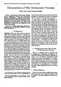
FIG. 1. Map showing the locations of GEOS station sites (triangles), epicenters (circles), and focal mechanisms of the Goodnow aftershock events used in this study. The tics indicate latitude (degree north) and longitude (degree west). The sizes of circles are proportional to the event magnitudes.
time-bandwidth parameter of 2v (e.g., Chave et al., 1987; Park et al. 1987). These multiple-taper windows simultaneously minimize both spectral leakage and variance and should generally yield higher confidences and frequency resolutions. The signal processing procedure can be briefly summarized as follows: (a) The fast Fourier transform (FFT) is applied to the time series obtained by applying MTW to the P or S wave train. The typical window lengths for P and S waves are 0.4 and 0.9 sec, respectively. For a few P-wave records from event 1016-0 we shortened the window length to 0.3 sec to avoid contamination by signals from 1016-1 (Table 1). (b) FFT and MTW are applied to time series prior to P arrivals to obtain moving-window RMS averages of reference ambient noise spectra. (c) At each station spectral ratios are computed for velocity amplitude spectra from larger events with respect to those of small events. When free of noise, the spectral ratios thus computed are the amplitude spectra of the deconvolved rupture pulses of the larger events. Figure 2 shows the results of the spectral analysis for signals from events 1016-0/1016-2 recorded by station G1H. The top left panel of Figure 2 shows, from the top trace to the bottom trace, the P-wave velocity spectra from event 1016-0 (M E = 2.4), 1016-2 (the Green's function event), and ambient noise. To make it easy to see the slopes of the spectral increase or decay, we also plotted guidelines (dashed lines) with arbitrary intercepts and slopes of ÷ 1 and - 1 , which are the slopes of the low- and high-frequency asymptotes of velocity spectra, had the path effects been removed. The top right panel shows the ratio of the P-wave spectrum from event 1016-0 to that from 1016-2. In this panel we also plotted a dashed guideline with an arbitrary intercept and a slope of - 2 , the slope of high-frequency asymptotes of the earthquake source spectra, according to the ~o-square source model (Brune, 1970). The bottom panels of Figure 2
823
R U P T U R E S OF G O O D N O W A F T E R S H O C K S
show, in the same order as in the top panels, the corresponding S-wave spectra and spectral ratios, together with the reference lines of slopes + 1, - 1, and - 2. Figure 3 shows, in the same manner as in Figure 2, results from events 1012/1016-2 at station G1H. The characteristics of spectra and spectral ratios from all the other stations are similar to those plotted in Figure 2 and are not plotted. In the following paragraphs we summarize the characteristics of the spectra and spectral ratios (please refer to those plotted for G1H in Figs. 2 and 3 as examples): (1) All of the amplitude spectra of P and S waves in this study are greater than those of reference noise by at least 20 dB at frequencies below the corner frequencies of the antialiasing filters (100 Hz in Figs. 2 and 3). The effects of ambient noise are therefore ignorable in this study. (2) At low frequencies, P-wave spectra increase with frequency at slopes that
glh 10 ° ~
P wave velocity spectra .:. ......., ........ , ........ ,
10-~ I i0-2
"~'~
1016-0/1016-2 1
|
//j! ..
"-\
O0
P wave spectral
........ , ........ ~ ........ , \ \ \
ratio
.....
\
10
\
('4
f
,o-. f
I \
13
\ 10
\
-6
10-7 r 0.1
glh 10 °
\ ........
,
........
,
......
I 10 frequency
,
........
100 (Hz)
1000
S wave velocity spectra . . . . . . . . J" < ....... '
10-'
........ ~ ' '
~..
0.1
,
........
0.1
~-'"I
1
O0
//
/ . x
(J
i0-~
/f
........
i
........
1 10 frequency
1016-0/1016-2
10 -2
v
=
S
I
, ~,,,,
100 (Hz)
wove
1000
spectral
ratio
........ ~ ........ ~ ........ , ....... \ \ \ \
('4 13
./
\
10" °~ .10
o
\
"s
\
104
\ \
10 .7
0.1
........ J
.................
1 10 frequency
'
100 (Hz)
...... 1000
O. 1
0.1
........
........ ' . . . . . . . ~ ..... 1 10 100 1000 frequency (Hz) ~
FIG. 2. P- and S-wave ground velocity spectra (in cm) and spectral ratios (dimensionless) at station G1H from events 1016-0 (M L = 2.4) and 1016-2 (M L = 1.6). (Top leflpanel:) P-wave velocity amplitude spectrum from event 1016-0 (top solid trace), 1016-2 (middle solid trace), and from the RMS average of the a m b i e n t noise (bottom solid trace). Dashed lines are guidelines with a r b i t r a r y intercepts and slopes of + 1 and - 1, which are the slopes of high- and low-frequency asymptotes of source spectra according to the u-square source model. (Top right panel) Ratio of P amplitude spectrum from 1016-0 with respect to t h a t from 1016-2 (solid line), and a dashed guideline with a n arbitrary intercept and a slope of - 2 , the latter being the slope of high-frequency asymptotes of the source spectra according to the co-square model. (Bottom left) S-wave velocity amplitude spectrum from event 1016-0 (top solid trace), 1016-2 (middle solid trace), and from the RMS average of a m b i e n t noise. (Bottom right) Ratio of S amplitude spectrum from 1016-0 with respect to t h a t from 1016-2. Dashed lines in the bottom panels are guidelines plotted in the same m a n n e r as in the top panels.
824
J. X I E E T A L . glh 100
P wave velocity spectra i
.~ .......
I
........
........
I
1012/1016-2 1 O0
......
........,
P wave spectral ratio ........ p, ........ ,
.......
\
10 -~
\
~ " I 0 -2 10 (%1
,-., i0-~ ®
.-,'z
10
-4
/i
/
\
-ECLI 0 -s 10-6
1 0 -7
........
0.1
glh 10 °
i
i
1 10 frequency
........
i
......
100
,
1000
........
,....
\
\
\
..... 100 1000 (Hz)
........ '
10
S wave spectral ratio ........~ ........~
%..
......
\
\
10-3
I 0 -4
........ '
frequency
10 -=
®
........ '
(Hz)
o
--,
O. 1
S wave velocity spectra
10 -1 ?
........
\
(N
//
1c
\
i
/
~ . 10 -~
E
10-~ 1 0 -7
0.1
........
i
........
i
........
i
1 10 100 f r e q u e n c y (Hz)
1000
0.1 0.1
........
i
........
i
1 10 frequency
.............
100 (Hz)
1000
FIG. 3. P- a n d S-wave ground velocity spectra (in cm) and spectral ratios (dimensionless) at station G I H from events 1012 ( M L = 3.1) and 1016-2 ( M L = 1.6). Spectra and spectral ratios are shown in the same way as in Figure 2, with event 1016-0 in Figure 2 replaced by 1012.
are generally slower than + 1. The increase continues until global peaks are reached at frequencies in between about 30 to 60 Hz, depending on the event size. Above the frequencies where these global peaks are located, the P-wave spectra decrease with slopes increasing in magnitude, which can be explained by an ~o-square source model. At frequencies of about 60 Hz the magnitudes of these slopes become greater than one, indicating the existence of a hard-rock P-wave fmax (cf. Cranswick et al., 1985). Some P-wave spectra, such as that from event 1012 and station G1H (upper left of Fig. 3, top trace), have local peaks at frequencies of about 90 Hz. Above 100 Hz, the P-wave spectra at high-gain stations decay with a slope of - 7 , the slope of the antialiasing filter. (3) At low frequencies, the S-wave velocity amplitude spectra increase with frequency at slopes of about + 1. At frequencies between 30 to 60 Hz where the P spectra reach global peaks, the S spectra also locally reach spectral peaks. At higher frequencies, however, the S spectra either decrease slightly or maintain about the same level until drastic increases occur near 90 Hz, resulting in global peaks at 90 to 100 Hz. These global peaks, as well as the local peak in P-wave spectrum from event 1012 at GIH mentioned in (2), are caused by the resonance of the geophone legs discussed by Cranswick et al. (1985).
R U P T U R E S OF G O O D N O W A F T E R S H O C K S
825
(4) Virtually all of the spectral ratios show the general trend of a decrease with increasing frequency at frequencies below about 50 to 60 Hz. This indicates that when the frequency increases the larger events have spectral fall-offs that are faster than that of the Green's function event. This is to be expected when the Green's function event is ~-like, in which case the spectral ratios plotted should resemble the source spectra of the larger events. According to the c0-square source model (Brune, 1970), the source spectra should be flat at low frequencies and should have a corner frequency, above which the spectra decrease at a slope of - 2 . In Figures 2 and 3, the source corner frequencies of the spectral ratios are somewhat ambiguous b u t should be somewhere below 30 Hz. Assuming a corner frequency of 20 Hz for event 1012, the expected corner frequency of event 1016-2 (Table 1) would be 63 Hz. Then, the source of 1016-2 would be effectively 5-like below about 50 Hz. We will study the source rupture process via a deterministic deconvolution, rather than by directly picking corner frequencies. (5) Above about 60 Hz the trend of decay in spectral ratios with frequency are gradually diminished or altered, and at frequencies of about 90 to 100 Hz there are sharp peaks resulting from the resonance mentioned in (3). It is important to note that the spectral divisions have not canceled the effect of this resonance near its peak. This implies that the resonance of the instrument legs does not linearly respond the ground motion. It is well known that the resonances of mechanical systems with damping can be physically unstable, with sudden "jumps" in their amplitude (Thompson, 1981). Of all the P records analyzed, only those from stations G1H and G4H provide amplitude spectra that have pronounced fmax effects at frequencies free of the instrument resonance effect. We have calculated the acceleration spectra for P waves at these two stations after removing the response of the antialiasing filter. Figure 4 shows, from the top trace to the bottom trace, the resulting acceleration amplitude spectra from events 1012, 1016-0, 1016-2 at G1H. For the convenience in comparison the latter two spectra have been artificially
P wave acceleration, glh 10 °
........
i
........
I
........
I
.....
~ 10 -2 -~ 10-5 .v. o--
~" i0-4 o 10 -5 10 -1
10 0
10 t
frequency
10 2
10 3
(Hz)
FIG. 4. Acceleration spectra at G I H from events 1012 (top), 1016-0 (middle), and 1016-2 (bottom). The antialiasing filter responses have been removed for all of the spectra, and the spectra from 1016-0 and 1016-2 have been artificially shifted downwards by 14 and 34 dB for the convenience of display. The fmax is estimated to be 57 Hz.
826
J. XIE E T A L .
shifted downward by 14 dB and 34 dB, respectively. In these traces, there appear to be sharp spectral fall-offs around 57 Hz. Cranswick et al. (1985) analyzed this phenomenon and attributed it to the existence of the fmax which, for station G1H, would be about 57 Hz. We have also estimated the P-wave fmax at station site G4 to be about 51 Hz. These are consistent with the values reported by Cranswick et al. (1985) for hard-rock sites in eastern Canada. THE EFFECTS OF FILTERING IN THE DECONVOLUTION OF RUPTURE PULSES
In order to reduce the effects of various sources of noise that generally grow with frequency, previous applications of the EGF method to study earthquake rupture processes have extensively used low-pass filtering (Mueller, 1985; Frankel et al., 1986; Li and Thurber, 1988; Mori and Frankel, 1990). In addition to ordinary filters, some authors also used the "water level correction," which functions as a low-pass filter at very high frequencies. In the last section we have found that the instrument resonance at 80 to 100 Hz is nonlinear and unstable and therefore adds an additional reason for low-pass filtering in this study. Based on the characteristics of the ground velocity spectra and spectral ratios summarized in the last section, we choose to use a seven-pole Butterworth low-pass filter with a corner frequency of 50 Hz. This filter should preserve the desirable source information indicated by the general increase of the spectral ratios with decreasing frequency below about 50 to 60 Hz and suppress the very high-frequency noise, especially the resonance with sharp peaks located between 80 and 100 Hz. This filter is also consistent with that used by Frankel et al. (1986), who used a 50 Hz filter partly for reducing the effects of non-identical paths of the larger events and the Green's function events. The latter effects are associated with spatial separations that are similar to those in this study ( - 200 m, cf. Table 1). The use of low-pass filtering will generally introduce two draw-backs in imaging the rupture processes, the first being an additional limit in time resolution besides that imposed by the sampling rate of the time series and the second being the distortion to the resulting time pulse. There has been a lack of discussion on these artifacts, and it is likely that portions of the previously reported rupture images have been affected by them. We shall therefore investigate, before the deconvolution is performed, both artifacts and the reduction of the second. Denoting the deconvolved time functions of a rupture pulse before and after the low-pass filtering by s(t) and s'(t), respectively, we have
s'(t) = [s(t) + n(t)]*f(t),
(1)
where n(t) and f(t) are time functions of noise and filter, and "*" stands for convolution. Assuming that after filtering and a Gaussian smoothing (Frankel et al., 1986) the noise is sufficiently suppressed, we can approximate equation (1) by
s'(t) ~ s(t)*f(t).
(2)
In general to achieve an efficient (i.e., non-oscillating) high-cut effect in the frequency domain, f(t) is not a positive function (e.g., Papoulis, 1962). For a
RUPTURES OF GOODNOW AFTERSHOCKS
827
given f(t), then, the " w i d t h " of s'(t) will depend on both the width of s(t) and the shape (e.g., slope, curvature) of s(t) in a complex manner. An example of this dependence is illustrated in Figure 5, where a synthetic triangular rupture pulse with a rise time (T1/2) of 0.0125 sec is plotted. Superimposed on this is a smoothed and broadened time pulse obtained by applying a seven-pole, Butterworth, 50 Hz low-pass filter to the triangular pulse. For simplicity we will call this filter "filter in this study" henceforth. The "rise time" of the low-pass filtered pulse can be defined either as the time difference between the zero crossing point of the pulse and the m a x i m u m point of the pulse (7~/2 in Fig. 5), or as the time difference between the minimum point and maximum point of the pulse (r~/2 in Fig. 5). As illustrated in Figure 5, r~/2 (0.0141 s) is usually closer to rl/2 (0.0125 sec) than r~/2 (0.0172 sec), and we shall use r~/2 exclusively in this article. To quantify the artifacts of the filter in this study, we have convolved two families of synthetic rupture pulses with this filter to study errors in r~/2 as compared to rl/2 . The first family of synthetic rupture pulses is characterized by linear rupture growths and the second by parabolic rupture growths (Herrmann, 1978). Assuming a symmetrical rupture and healing, these two families of ruptures approximate the "w-square" and the "c0-cube" source models, respectively (e.g., Brune, 1970, Savage, 1972). For both families of ruptures we have calculated r~/2 for rl/2 ranging from 0.003 to 0.03 sec. Figure 6 shows the resulting rl/z-r~/2 relations for both families of rupture pulses. At short r{/2 errors in r~/2 (i.e., r~/2 - rl/2) are large for both curves: when r~/2 equals to
I
I
I
O. 5 "D
2, E ¢B 0
-0,5
--
, , ,,***,lJ*
O. O1
J,,,,,
O. 03
,I,
,,,,
O. 05
time
, , , , I , , , , , , , , ,
O. 07
O. 09
Csec]
FIG. 5. An example of artifacts caused by low-passfiltering in deconvolvingrupture pulses. The triangular pulse is a synthetic rupture pulse with a rise time, rl/2 of 0.0125 sec. The smoothed, broadened curve is the convolution of the synthetic pulse with a seven-order, 50 Hz Butterworth low-pass filter, ri/2, the time difference between zero crossing and maximum point of the broadened curve, is 0.0141 sec, whereas r~/2, the time difference between the minimum and maximum point of the broadened curve, is 0.0172 sec..
828
J. X I E E T A L .
0.095 sec, the relative errors in T~/2 for both types of ruptures are greater than 100 per cent. As r'~/2 increases, the errors for both families of ruptures decreases with steep slopes. When T~/2 equals to 0.011 sec, the relative errors in r~/2 decrease to about 20 per cent and 12 per cent for linear and parabolic rupture growths, respectively. At larger r~/2 the relative errors vary between + 10 per cent and + 15 per cent for linear ruptures, and between - 4 per cent and + 5 per cent for parabolic ruptures. To test the validity of equation (2), we have also convolved the filter in this study with rupture pulses in the presense of a synthetic "resonance noise." The latter is constructed by passing white noise, with DC level the same as that of synthetic rupture, through a Gaussian filter centered at 90 Hz with a half width of 10 Hz. The resonance effect can be reasonably modeled in this way (e.g., Thompson, 1981). The resulting T~/2 differ by less than 1 percent from those calculated in the absence of noise. When r~/2 are less t h a n about 0.011 sec, the steep slopes (from asymptotically + oo to less t h a n + 2) of both curves in Figure 6 make the calculations of rl/2 using r~/2 very unstable, since a small error or uncertainty can be greatly amplified due to these slopes. Taking for example, an uncertainty in r~/2 of 0.0025 sec (the sampling interval of the high-gain instruments in this study), the uncertainty in rl/2 may well be greater than 100 per cent for T~/2 _< 0.011 sec. This conclusion can be extended to a general case: when the reading of r~/2 differs from 0 . 5 / f c by about 10 per cent or less, f~ being the corner frequency of the low-pass filter, the rise time (T1/2) values are practically unresolvable in the presense of noise or uncertainty. The resolution limits thus imposed on rl/2 is 0.9 times and 1.0 times of 0.5/f~ for linear and parabolic rupture growths. Thus in practice one must trade-off the desired resolution in rise time with the fidelity, the latter being obtained using low-pass filter to suppress noise.
O. 03
l l l l l l l l
I
'
'
I I I '
t
'
I I 't
i
I I I
I t ~ ' ~
0.02 U @
-~ 0.01
I l l l l l l
0
O. O1
tau'l/2
O. 02
O. 03
[~ec]
FIG. 6. Real rise T time versus a p p a r e n t "rise t i m e " r~/2 measured on synthetic linear a n d parabolic r u p t u r e pulses before and after low-pass filtering, r'{/2 is defined as in Figure 5.
RUPTURES OF GOODNOW AFTERSHOCKS
829
For greater 7~/2 readings, 71/2 may be calculated using the 71/2 - T~/2 relationships in Figure 6. ~1/2 thus obtained will be slightly model dependent but will be nevertheless closer to the true ~1/2, as compared to 7~/2. RUPTURE PROPERTIES OF THE LARGER ( M L > 2.1) AFTERSHOCKS
Assuming that the source of event 1016-2 ( M L = 1.6) can be treated as a d-like impulse at frequencies below about 50 Hz, and denoting the far-field displacement from a larger event and from event 1016-2 by u~(x, t) and u n (x, t), respectively, we have (Appendix of this paper)
u.(x, t) = -- oGUn (x,t)*s(t),
(3)
where tt is the shear modulus on the fault, Mov is the seismic moment of the Green's function event, and
s(t)= f
//)(x',t+to+--
ax'- c
(4)
is the source pulse. The notation on the right hand side of equation (4) is defined in the Appendix. We deconvolved the source pulses, s ( t ) , of events 1012, 1016-0, and 1016-1. The deconvolution process is the same as that of Frankel e t a l . (1986). In particular we have used the seven-pole, 50 Hz low-pass filter discussed in detail in the last section. Figures 7a and b show the P and S waves from event 1016-0 and the Green's function events, and the deconvolved rupture pulses. Above each P- or S-wave trace are the event code, magnitude, the station code, wave type, and peak ground velocity. Above each deconvolved rupture pulse, the epicenter-station azimuth and the peak value in s -1 are given. The window lengths used in Figures 7a and b are the same as those described in Section 3. Despite the wide coverage of azimuths of the stations (three quadrant), the deconvolved rupture pulses in Figures 7a and b are similar and the peak values of the deconvolved rupture pulses differ by less t h a n 30 per cent. This indicates that the rupture of event 1016-0 is nearly circular. Figures 8a and b show the P and S waveforms from events 1012 and 1016-2 and the deconvolved rupture pulses for event 1012. Again, most of the deconvolved pulse widths are similar, and most of the peak values of the deconvolved rupture pulses agree with one another within about 40 per cent. However, two exceptions can be observed, the first being the somewhat wider pulse width of deconvolved P at G2H and the second being the considerable greater amplitude of the deconvolved S at G4L. These exceptions are likely due to the noise problem r a t h e r t h a n due to source directivity, since the P and S do not vary systematically. The first exception may be associated with perturbed response of the instrument whose low-frequency (< 0.3 Hz) zero line drift is visible on the P traces from 1012 before and after deconvolution (panels second from top in Fig. 8a). We conclude that the rupture of event 1012 is also nearly circular. We measured the 7~/2 values as defined in the last section for all of the deconvolved traces from events 1012 and 1016-0, the resulting values are listed
830
J. XIE E T A L . 1016-0, M1=2.4, glh, P wave 0.0036 c m / s
1016-2, M1=1.0, glh, P wave 0.0012 c m / s
deconvolved pulse, Az.=325 317.7
1016-0, M1=2.4, g2h, P wove
1016-2, M1=1.6, gZh, P wave
0.0022 cm/s
0.00074 cm/s
deconvolvsd pulse, Az.=120 272.,7
0.1 sac
1016-0, M1=2.4, 931, P wave 0.0088 c m / s
0.1 se¢
1016-2, M1=1.6, 931, P wave 0.0028 c m / s ¢
1016-0, M1=2.4, g4h, P wave 0.01() c m / s
0.1 sea
1016-2, M1=1.6, g4h, P wove 0.0042 c m / s
~
se¢
deconvolved pulse, Az.=g6
~
308.5 sec
dsconvolvsd pulse, Az.=18
~
296.0 se¢
(a)
1016-0, M1=2.4, glh, S wove 0,015 ¢rn/s
1016-2, Id1=1.6, glh, S wove 0.0064 c m / s
deconvolved pulse, Az.=S25 293.3
1616-0, M1=2.4, g2h, $ wave 0.016 ¢m/s
1016-Z, M1=1.6, g2h, $ wave 0.0038 ¢rn/s
de¢onvolved pulse, Az.=120 298.8
1016-0, M1=2.4, gSI, $ wave 0.015 a m / s
1016-2, M1=1,6, 931, S wave 0.0033 a m / s
deconvolved pulse, Az.=96 553.7
M1=2.4, g4h, $ wave 0.012 ¢rn/s
1016-2, M1=1°6, 04h, • wove 0,0035 c m / s
deconvolved pulse. Az.=tS 376.2
1016-0,
(b) FIG. 7. (a) P waveforms from event 1016-0 (left traces), 1016-2 (middle traces), and r u p t u r e pulses obtained by deconvolving the P-wave signal of event 1016-2 from 1016-0 (right traces). Each row shows, from top to bottom, the traces from station sites G1, G2, G3 and G4. Above each P-wave plot are the event code and magnitude, the station code, wave type and peak velocity in cm/sec. Above each deconvolved r u p t u r e pulses are t h e epicenter-station azimuth in degrees and peak value in s-1. (b) S waveforms from events 1016-0 and 1016-2, and the corresponding deconvolved rupture pulses for event 1016-0. Plotted in the same way as in Figure 7a where P signals are plotted.
R U P T U R E S OF G O O D N O W A F T E R S H O C K S 1012, M1:3.1, glh, P wove 0.016 cm/s
1016-2, M1=1,6, glh, P wove 0.0013 crn/s
831
deconvolved pulse, Az.=325 1249,8
~
sec
1012, M1=3.1, g2h, P wave 0.0047 cm/s
1016-2, M1=1.6, g2h, P wave 0.00074 crn/s
deconvolved pulse. Az.--120 846.9 0.05 sec
1012, M1=3.1, g31, P wave 0.0,57 cm/s
1016-2, M1=1.6, g31, P wave 0.0028 cm/s
deconvolved pulse, Az.=96 1222.5
1012, M1=5.1, g41, P wave 0.051 am/s
1016-2, M1=1.6, g41, P wove 0.0042 cm/s
~
sec
deconvolved pulse, Az.=18 1069.5
~
sec
(a)
1012, M1=3.1, glh, S wove 0.037 cm/s
1016-2, M1=1.6, glh, S wove 0.0064 cm/s
0.2 see
1012, M1=3.1, g21, S wove 0.06 cm/s _
_
~
.
2
deconvolved pulse, Az.=325 570.8
0,2 sea
1016-2, M1=1.6, g21, $ wove i0,0030 cra/s sea
~
2
s
e
c
deoonvolved pulse, Az.=120 733.2 . ~
1012, Ml=3,1, g31, S wove 0.076 crn/s
1016-2, M1=1.6, g31, $ wove 0.00,$3 cm/s
deconvolved pulse, Az.=96 889.7
1012, M1=5.1, g41, S wove 0.038 ¢m/s
1016-2, M1=1.6, g41, S wove 0.0053 crn/s
deconvolved pulse, AZ.=18 1049.4
o.,zo
sec
o. .o
FIG. 8. (a) P waveforms from events 1012 and 1016-2, and the deconvolved rupture pulses for event 1012. Plotted in the same way as in Figure 7a. (b) S waveforms from events 1012 and 1016-2, and the deconvolved rupture pulses for event 1012. Plotted in the same way as in Figure 7b.
832
J. XIE E T A L .
in Table 3. They generally differ from 0.01 sec (0.5/fc) by more than 20 per cent and hence are free of the instability problem discussed in the last section. For each event, the fault radius r, and the stress drops are calculated using the following relationships (Boatwright, 1980, Keilis-Borok, 1959): T1/2 Fr r=
(5)
1 - (VrSinO/c)
and 7Mo
= 16r--
(6)
where T1/2 is the corrected rise time, c and vr are the velocities of wave and rupture, respectively. 8 is the take-off angle. We use a vr of 0.90 of the local shear-wave velocity and assume an average 0 of 45 ° for both P and S wavetrains. For the larger event the seismic moment Mo, in units of Mo G, can be obtained by calculating / s ( t ) d t (Aki and Richards, 1980). In a waveform modeling study, Liu et al. (1991) have estimated the P and S velocities near the fault to be 6.6 km/sec and 3.82 km/sec, respectively, and Mo ~ of event 1016-2 to be 1.52 x 10 is dyne-cm. Using these values as well as equations (5) and (6), and assuming that the source pulses of event 1016-2 are 6-like, we calculated M o and Aa for events 1012 and 1016-0. The results are summarized in Table 4, where the rupture parameters estimated using r~/2 - rl/2 relationships for linear and parabolic rupture growth are listed separately. Our pre-
TABLE 3 3-~/2 Measurements 1012
1016-0
1016-1
Station/Phase
(sec)
(sec)
(sec)
G1/P G2/P G3/P G4/P
0.0140 0.0219 0.0163 0.0147 0.0203 0.0125 0.0204 0.0220
0.0133 0.0149 0..0157 0.0115 0.0120 0.0133 0.0131 0.0134
0.0120 0.0120 0.0108" 0.0117 0.0123 0.0137 0.0114 0.0120
G1/S
G2/S G3/S G4/S
*Not used for results in Table 4.
TABLE 4 RUPTURE PROPERTIES OF THE THREE ( M L ~ 2 TO 3) GOODNOW AFTERSHOCKS
Event Code
ML
Fault Radius* (m)
Fault Radius~ (m)
(10 is dyne-cm)
Mo
Stress Drop* (bar)
Stress Dropt (bar)
1012 1016-0 1016-1
3.1 2.4 2.1
117.0 _+ 46.9 85.1 +_ 24.2 78.8 +_ 25.0
138.1 + 56.6 99.0 +_ 28.2 91.4 +_ 29.1
27.47 +_ 4.62 7.03 + 0.52 3.67 _+ 0.84
15.5 +_ 14.8 8.2 -I-_7.9 4.7 +_ 3.4
9.7 -I--9.4 5.2 _+ 5.1 3.0 + 2.2
* O u r preferred parameters, calculated using r[/2 - r:/2 relationship for linear rupture growths. *Parameters calculated using r~/2 - rl/2 relationship for parabolic rupture growths.
R U P T U R E S OF G O O D N O W A F T E R S H O C K S
833
ferred results are those obtained assuming a linear rupture growth since its amplitude spectra approximates the ~-square source model, which may be statistically more appropriate than the ~-cube model. We have also deconvolved rupture pulses of event 1016-1 using the empirical Green's function method with a shorter window length (0.3 sec) to reduce the contamination by signals from event 1016-0 which occurred only 0.6 sec earlier. The T~/2 m e a s u r e m e n t s are also listed in Table 3. Since seven of the r~/2 measurements differ from 0.01 sec by about 20 per cent or less, the widths of rupture pulses from this event may be close to the resolution limit imposed by the 50 Hz low-pass filtering. One of the apparent rise time readings (G3L, P) is about 108 per cent of 0.01 and is not used to avoid error in estimating 71/2. The resulting parameters for event 1016-1 using the remaining seven P and S traces are listed in Table 4. We note here that the low-pass filtering does not affect the estimation of seismic moments that depend only on low-frequency content of the source information. The seismic moment of event 1012 has also been estimated by matching low-frequency displacement spectral level and by waveform modeling (Liu et al., 1991), and the results are identical to that in Table 1. Comparing the results in Table 4 with those obtained for the main shock (N~b~lek and Su~rez, 1989) and for the microearthquakes in California (Frankel et al., 1986; Mori and Frankel, 1990) and in Hawaii (Li and Thurber, 1988), we found that the fault radii in Table 4 are generally smaller than those of both the main shock and of the events in California and Hawaii. The stress drops in Table 4 are dependent on the sizes of the events and are considerably smaller than those estimated for the main shock (115 to 670 bars), even after we take into account the large uncertainty in the latter estimates caused by uncertainty in path Green's function. If an assumption is made that the static stress drops reflect the strain energy accumulation and the absolute stress, we may interpret the generally lower stress drop of the aftershock as being caused by the release of large amount of strain energy during the main shock. This stress drop variation is similar to those reported by Boore and Atkinson (1989) for the Nahanni and Miramichi earthquake sequences. Another stress drop variation, similar to that reported in this study, is reported by Mori and Frankel (!990) for the 1986 North Palm Springs California earthquake ( M L = 5.9) sequence. During that sequence the stress drops decrease from above 80 bars in a foreshock and 50 to 100 bars in the main shock, to between about 3 to 30 bars in the aftershocks in the hypocentral area. If 115 bars, the lower bound of the estimated stress drop, is adopted for the Goodnow main shock, the stress drops during these earthquake sequences being compared overlap one another, each varying by a factor of 5 or more. Another interesting comparison can be made using the previously reported stress drops, estimated with the EGF method, for simple crack-like ruptures during microearthquakes (M z - 2 - 4 ) in different areas. The result of this comparison is listed in Table 5. For five events belonging to a swarm near Anza, California, the stress drops are estimated to be 11 to 54 bars, with a median of 38 bars (Frankel et al., 1986). For the simple crack-like ruptures in the foreshock/aftershock sequence ( M L - 2 to 4) before and after the North Palm Springs earthquake, the stress drops span a much wider range (between 3 and 82 bars); the median (23.5 bars), however, is similar to other medians in the interplate sequences in Table 5. Li and Thurber (1988) studied the stress drop of a simple crack-like microearthquake ( M L ~ 2) in Hawaii and obtained a value of 16.5 bars, but it is likely that this value is
834
J. XIE E T A L .
~>
© ¢*q
o
~9
© Z O
¢0
©
q~
RUPTURES OF GOODNOW AFTERSHOCKS
835
somewhat underestimated since the reported rise times are similar to 0.5/fc, fc being the corner frequency of the low-pass filter (15 to 25 Hz) used in that study. The stress drops in Table 4 (4.7 to 15.5 bars, with a median of 9.5 bars) are generally lower than those of the other areas, despite the fact that the Goodnow aftershocks occurred in an intraplate environment. The medians of the stress drops calculated for each of the event groups in Table 5 vary by factors of up to 4, whereas the stress drops within each source area vary by factors ranging between 3 and 27. SOURCE MULTIPLICITY: SEPARATE RUPTURES OF PATCHES
Event 1016-0 is followed by 1016-1, which provided recognizable P and S phases on five of the eight records. The polarities of the first few cycles of these five P and S phases are very similar to those of the corresponding P and S phases from event 1016-0, indicating similar focal mechanisms. The corresponding time delays between the same phases from the two events are in the range of 0.600 _+ 0.005 sec. It has been documented that complex rupture processes occurred during some microearthquakes in California and Hawaii (Frankel et al., 1986; Li and Thurber, 1988; Mori and Frankel, 1990). Interestingly, the 19 October 1985, Ardsley, New York, earthquake (M = 4.0) is composed by events which are also separated by roughly 0.6 sec (Barstow et al., 1988), although due to poor azimuthal coverage the relative locations of these events are not determined. It is therefore interesting to investigate whether the ruptures of events 1016-0 and 1016-1 have occurred during one complex rupture process (which would indicate the variability and complexity during small earthquakes in this area), or whether they are ruptures of independent, simple patches. The key to this investigation is the precise relative location of these two events. Location A l g o r i t h m
The algorithms for determining the relative locations of two events have been discussed by Poupinet et al. (1984) and Ito (1985). Their methods involve calculating cross-correlations of moving window spectra. AT, the difference in the origin times of events 1016-0 and 1016-1 is small (0.60 sec), and we have therefore designed a simple and fast deconvolution technique to determine their relative locations, assuming that both events are close to 1016-2, the Green's function event. The theoretical basis of this algorithm is given in Appendix. In the following paragraphs we briefly describe this algorithm. We chose window lengths T W and T{~ of 0.3 and 0.9 sec, which are used to window the time series unG(x, t) from the Green's function event and Un(X, t) from events 1016-0 and 1016-1, respectively. These window lengths satisfy equation (A9) and avoid the S-wave contamination on vertical components, since a T W of 0.9 sec is less than the minimum S-P travel time difference at all of the stations (about 1.0 sec). For each component of motion at each station we deconvolve u~G(X,t) from u'(x, t). At the kth station P~, the time difference between the onsets of P waves from events 1016-0 and 1016-1 is then measured. Similarly we define and measure S k for the S waves. For each of the available nonrepeat station pair (k, k + 1)(k = 1, 3, 5 , . . . ), we define a quantity
f ~r~ = ~ ( Sh
Sk+l Pk+l
for i = 1 (k = 1,3,5, ) fori=2 ....
(7)
836
J. XIE ETAL.
From equation (A17), [V'TP(xk,x') Ari~ =
V, TS(xk,x, )
v ' T s ( x k + l , x ' ) ] 'Sx'
for/= 1
V'TP(xk+l,x')]
for i = 2
5x'
, ( k = 1 , 3 , 5 .... ),
(8) where 5x' is the location of event 1016-1 relative to that of 1016-0. Defining an integer variable m(i, k) such that m ( i , k ) = i + (k - 1 ) , i = 1 , 2 a n d k = 1 , 3 , 5 , . . . ;
(9)
we can rewrite (8) as I
Arik = A7 m = Gmj~xj, j = 1,2,3,
(lO)
where for m ( i , k)li= 1
(11) GraY:
~
~xj
[TS(xk,x, )
TP(xk+l,X')]
for m ( i , k) li= 2
Now we can define and solve a least-square problem Ilr-G
Sx'll2 = rain
(12)
to obtain 5x'. The cross-use of P and S in the definition of Ar~k in equation (7) ensures that the G matrix has large elements and thereby stabilizes the least-square problem. Result: Location of Event 1016-1 Relative to 1016-0
Figure 9 shows the P and S H components of u~(x, t) after deconvolution of Una(X, t) (i.e., dn(x, t) in equation A13) at all of the four stations. We measured Arlk and solved the least-square problem (equation 12), using the same velocity structure as in Section 5. The resulting 5x', is ~x'T=
{22,180,- 45} (meters),
(13)
with the three components defined along the north, east and vertical (downwards) directions. The model variance of 5x' is estimated to be in the order of centimeters. To access the upper bound of the real errors, we generated a series of "errors" in 5r m with absolute values of 0.005 sec (twice of the sampling interval of most of the instruments involved). All of the possible combinations of the signs of these errors were tested. The resulting errors in 15x'l are generally small (of tens of meters), the largest being 122 m. Using these, we have 15x'l = 190 +_ 122 m, the error being most likely overestimated. Using a AT of 0.60 sec and assuming a rupture propagation from hypocenter of event 1016-0 to that of 1016-1, the rupture velocity would be 0.05 +_ 0.03 times the local shear-wave velocity of 3.82 km/sec. This is unreasonably low compared to 0.8 to 1.0 times of local shear velocities previously obtained for complex ruptures during microearthquakes (Frankel et al., 1986, Li and Thurber, 1988). We
R U P T U R E S OF G O O D N O W A F T E R S H O C K S glh, P wave
g2h, P wave
g31, P wove
94h, P wave
837
(a) glh,
g2h, S wave
S wave
g4h, S wave
g 3 l , $ wave
(b) FIG. 9. Deconvolved P and S signals (dn(x, t)) containing rupture pulses from events 1016-0 and 1016-1. The window lengths used~n deconvolution is 0.9 sec for u'_(x, t), signals from events 1016-0 and 1016-1, and is 0.3 sec for u n (x, t), signals from the Green's l~unction event. (a) Deconvolved P pulses. (b) Deconvolved S pulses,
therefore interpret the ruptures of events 1016-0 and 1016-1 as being distinct, each rupture due to the failure of a small patch. Although the second rupture is not as well resolved as the first, it is reasonable to assume, based on deconvolved rupture pulses (see Fig. 9), that it is also nearly symmetrical. The failure of these two patches are independent in the sense that they are not subevents of one complex rupture with a reasonable rupture velocity. Assuming a causality between the two failures, the propagation of this causality is on the order of hundreds of meters per second, similar to those involved in "silent earthquakes" (Beroza and Jordan, 1990). The characteristic length of the area separating the two small patches is about 26 m, roughly 0.2 times of those of the broken patches. CONCLUSIONS AND DISCUSSION
GEOS data from four aftershock events ( M L - 1 to 3) of the 1983 Goodnow, New York, earthquake, recorded on four hard-rock sites a few kilometers away from the epicenters, are collected and analyzed. The complexity of ground velocity spectra at frequencies of up to 100 Hz were analyzed using a set of multiple-taper windows. We resolved P-wave fm~ of 51 and 57 Hz for two sites. We found that using a small ( M L = 1.6) event as the Green's function event, the deconvolved P and S signals from the larger events are dominated by source energy radiation at frequencies below 50 to 60 Hz and are severely contaminated by instrument resonances at frequencies between about 80 and
838
J. X I E E T A L .
100 Hz. These resonances appear to be unstable (event variable) and nonlinear, adding an extra reason for applying low-pass filtering in using the empirical Green's function (EGF) method. We analyzed the trade-off between resolution and fidelity in studying earthquake rupture processes with the EGF method due to the use of low-pass filtering. Denoting the corner frequency of the filter by fc, we found that when the apparent "rise time" measured on a deconvolved and low-pass filtered rupture pulse differ from 1/2 fc by less than 10 per cent, the real rise time is virtually unresolvable. For longer apparent rise times, the reduction of the artifact in rise time measurements is slightly dependent on the rate of rupture growth. In interpreting real data a linear rupture growth is our preferred rupture growth model. Applying the EGF method to image ruptures of the larger ( M L - 2 to 3) aftershocks, we found that these ruptures are simple crack-like, with small fault radii (70 to 110 m), and stress drops between 5 and 16 bars. Two of the events ( M L ~ 2) studied are separated by a small (0.6 sec) time interval. We extended the deconvolution algorithm to precisely locate these events and to estimate the propagation velocity of the possible causality. This velocity is found to be 0.05 +_ 0.03 times of the local S-wave velocity. Therefore we interpret the two ruptures as being separate, rather than being connected into one complex rupture process. Interestingly, the area separating the two ruptures has a diameter that is only 0.2 times of those of the rupturing areas. Comparing the stress drops obtained in this study with those estimated for the Goodnow main shock (m b = 5.1) suggests that the stress drops in the Goodnow earthquake sequence decreases from above 115 bars in the main shock to 5 to 16 bars in the aftershocks. This is similar to the decrease of the stress drops in the Nahanni earthquake sequence (M b = 5.0 to 6.5) and in the North Palm Springs earthquake ( M L = 5.9) sequence. The stress drops of simple crack-like microearthquakes in the Goodnow area and areas near Anza and North Palm Springs, California, are all significantly variable (by a factor of 3 to 27) within the same source zone. The median value of the stress drops of the Goodnow aftershocks is lower than those estimated for the other earthquake sequence by a factor of 2 to 4, despite the fact that the Goodnow aftershocks occurred in an intraplate environment whereas other earthquake sequences occurred in interplate environments. Therefore, even for the simple crack-like microearthquake ruptures, the stress drops within an intraplate or interplate area do not seem to have a tendency to cluster around some constant values, with the value in intraplate areas higher than that in interplate areas. We note, however, that the data base is still small and further analysis of the growing high-quality data base should be performed in the future to examine this issue on a more solid ground. A bi-product of this study is the modification or development of the deconvolution/relative location algorithms, which can be applied to both the study of clustered earthquake events and the studies of the ripple firing or explosion/spall processes in explosion discriminations (e.g., Baumgardt and Ziegler, 1988). ACKNOWLEDGMENTS We t h a n k Dr. B. J. Mitchell for his support, discussion, and encouragement t h r o u g h o u t this research. T h a n k s are due to Drs. C. Chester and Gou-Bin Ou for t h e i r fruitful discussions and to Dr.
RUPTURES OF GOODNOW AFTERSHOCKS
839
Alan Chave for his kindness in providing us computer codes for multiple-taper window spectral analysis. Constructive reviews by Dr. A. Mendez and D. Boore helped us to improve the quality of this paper. This research was partly supported by the Advanced Research Projects Agency of the Department of Defense and monitored by the Air Force Geophysics Laboratory under contracts F19628-89-K-0021 and F19628-K-0040. REFERENCES Aki, K. and P. G. Richards (1980). Quantitative Seismology: Theory and Methods, W. H. Freeman, San Francisco. Barstow, N., J. A. Carter, P. W. Pomeroy, and G. H. Sutton (1988). Near-regional waveforms: selected observations from two eastern North American earthquake sequences, Seism. Res. Lett. 59, 189-196. Baumgardt, D. R. and G. R. Ziegler (1988). Spectral evidence for source multiplicity in explosions: application to regional discrimination of earthquakes and explosions, Bull. Seism. Soc. Am. 78, 1773-1795. Beroza, G. C. and T. H. Jordan (1990). Searching for slow and silent earthquakes using free oscillations, J. Geophys. Res. 95, 2485-2510. Boatwright, J. (1980). A spectral theory for circular seismic sources: simple estimates of source dimension, dynamic stress drop, and radiated energy, Bull. Seism. Soc. Am.~ 70, 1-28. Boore, D. M. and G. M. Atkinson (1987). Stochastic prediction of ground motion and spectral response parameters at hard-rock sites in eastern north America, Bull. Seism. Soc. Am. 77, 440-467. Boore, D. M. and G. M. Atkinson (1989). Spectral scaling of the 1985 to 1988 Nahanni, Northwest Territories, earthquakes, Bull. Seism. Soc. Am. 79, 1736-1761. Borcherdt, R., J. B. Fletcher, E. G. Jensen, G. L. Maxwell, J. R. VanSchaack, R. E. Warrick, E. Cranswick, M. J. S. Johnston, and R. McClearn (1985). A general earthquake observations system (GEOS), Bull Seism. Soc. Am. 75, 1783-1826. Brune, J. N. (1970). Tectonic stress and the spectra of seismic shear waves from earthquakes, J. Geophys. Res. 75, 4997-5009. Chave, A. D., D. J. Thomson, and M. E. Ander (1987). On the robust estimation of power spectra, coherences, and transfer functions, J. Geophys. Res. 92, 633-648. Cranswick, E., R. Wetmiller, and J. Boatwright (1985). High-frequency observations and source parameters of microearthquakes recorded at hard-rock sites, Bull. Seism. Soc. Am. 75, 1535-1567. Frankel, A., F. Fletcher, F. Vernon, L. Harr, J. Berger, T. Hanks, and J. Brune (1986). Rupture characteristics and tomographic source imaging of M L - 3 earthquakes near Anza, southern California, J. Geophys. Res. 91, 12633-12650. Geller, R. J. and C. S. Mueller (1980). Four similar earthquakes in central California, Geophys. Res. Lett. 7, 821-824. Hanks, T. C. (1982). fmax, Bull. Seism. Soc. Am. 72, 1867-1879. Hanks, T. C. and D. M. Beore (1984). Moment-magnitude relations in theory and practice, J. Geophys. Res. 89, 6229-6235. Hartzell, S. H. (1978). Earthquake aftershocks as Green's functions, Geophys. Res. Lett. 5, 1-4. Herrmann, R. B. (1978). A note on causality problems in the numerical solution of elastic wave propagation in cylindrical coordinate systems, Bull. Seism. Soc. Am. 68, 117-123. Hutchings, L. and F. Wu (1990). Empirical Green's functions from small earthquakes: a waveform study of locally recorded aftershocks of the 1971 San Fernando earthquake, J. Geophys. Res. 95, 1187-1214. Ito, A., (1985). High-resolution relative hypocenters of similar earthquakes by cross-spectral analysis method, J. Phys. Earth 33, 279-294. Kanamori, H. and D. L. Anderson (1975). Theoretical basis of some empirical relations in seismology, Bull. Seism. Soc. Am. 65, 1073-1095. Kanameri, H. and C. Allen (1985). Earthquake repeat time and average stress drop, in Earthquake Source Mechanics, S. Das, J. Boatwright, and C. H. Sholz (Editors), American Geophysical Union Monograph 37, Washington, D.C., 227-235. Keilis-Borok, V. I. (1959). On the estimation of the displacement in an earthquake source and of source dimensions, Ann. Geofis., 12, 205-214. Li, Y. and C. H. Thurber (1988). Source properties of two microearthquakes in Kilauea volcano, Hawaii, Bull. Seism. Soc. Am. 78, 1123-1132.
840
J. XIE E T AL.
Liu, Z., R. B. Herrmann, J. Xie, and E. D. Cranswick (1991). Waveform characteristics and focal mechanism solution of five aftershocks of the 1983 Goodnow, New York, earthquake by polarization analysis and waveform modeling, Seism. Res. Lett. (in press). Mori, J. and A. Frankel (1990). Source parameters for small events associated with the 1986 North Palm Springs, California, earthquake determined using empirical Green functions, Bull. Seism. Soc. Am. 80, 278-295. Mueller, C. (1985). Source pulse enhancement by deconvolution of an empirical Green's function, Geophys. Res. Lett. 12, 33-36. N~b~lek, J. and G. Sufirez (1989). The 1983 Goodnow earthquake in the central Adirondacks, New York: rupture of a simple, circular crack, Bull Seism. Soc. Am. 79, 1762-1778. Nuttli, 0. W. (1983). Average seismic source-parameter relations for mid-plate earthquakes, Bull. Seism. Soc. Am. 73, 519-535. Officer, C. B. (1974). Introduction to Theoretical Geophysics, Springer-Verlag, New York, 385 pp. Papageorgiou, A. S. and K. Aki (1983). A specific barrier model for the quantitative description of inhomogeneous faulting and the prediction of strong ground motion. I. Description of the model, Bull. Seism. Soc. Am. 73, 693-722. Papoulis, A. (1962). The Fourier Integral and Its Applications, McGraw-Hill, New York, 318 pp. Park, J., C. R. Lindberg, and Vernon, F. L. (1987). Multitaper spectral analysis of high-frequency seismograms, J. Geophys. Res. 92, 12,675-12,684. Poupinet, G. W., W. L. Ellsworth, and J. Frechet (1984). Monitoring velocity variations in the crust using earthquake doublets: application to the Calaveras fault, California. J. Geophys. Res. 89, 5719-5731. Ruff, L. J. (1987). Tomographic imaging of seismic sources, in Seismic Tomography, G. Nolet (Editor), Reidel, Dordrecht, 339-366. Savage, J. C. (1972). Relation of corner frequency to fault dimensions, J. Geophys. Res. 77, 3788-3793. Seeber, L. and J. G. Ambruster (1986). A study of earthquake hazards in New York and adjacent areas, Final report covering the period 1982-1985, Report to the Nuclear Regulatory Commission, NUREG/CR-4750, Washington, D. C., pp. 98. Somerville, P. G., and J. P. McLaren, L. V. LeFevre, R. W. Burger, and D. V. Helmberger (1987). Comparison of source scaling relations of eastern and western north American earthquakes, Bull. Seism. Soc. Am. 77, 322-346. Thompson, W. T. (1981). Theory of Vibration with Applications, Prentice-Hall, Englewood Cliffs, New Jersey, 467 pp. APPENDIX: SOME USEFUL RELATIONSHIPSIN DECONVOLUTION I n this a p p e n d i x we derive e q u a t i o n s (3), (4), a n d (8). F o l l o w i n g A k i a n d R i c h a r d s (1980) a n d R u f f (1987) a n d after some m a n i p u l a t i o n , t h e far-field displacement, u~(x, t) c a n be expressed as
u~(x,t) = t~pqg~pq(X,X'o)h(t-
T(x,x'o))*
b
x',t + - c
dE(x'), (A1)
w h e r e t h e s u m m a t i o n c o n v e n t i o n on t h e d u m m y indices h a s b e e n used, x, x' are vectors specifying t h e locations of t h e o b s e r v a t i o n p o i n t a n d source point, respectively; x' 0 is a reference p o i n t on t h e f a u l t p l a n e Z(x'); a n d ~npq is a " u n i t m o m e n t " d e s c r i b i n g t h e g e o m e t r i e s of slip dislocation a n d f a u l t g e o m e t r y . T(x, x') is t h e t r a v e l t i m e f r o m x' to x w i t h w a v e velocity c. ~ is the elastic s h e a r m o d u l u s on t h e fault, g~pq(X, x'), ( h ( t - T(x, x')) are p a r t i t i o n e d far-field G r e e n ' s f u n c t i o n defined via Gnp, q ( X , x ' , t ) ~ g n p q ( X , X ' ) h ( t -
where
T(x,x')),
G~p(x,x', t) is t h e g e n e r a l form of G r e e n ' s function.
(A2) D(x', t) is the
R U P T U R E S OF G O O D N O W A F T E R S H O C K S
841
dislocation slip function on the fault Z(x'), r o = Ix - x' o I, Ax' = x' - X'o, and is the unit vector pointing at the direction of (x - x~). The conditions for (A2) and (A1) to be valid are 1 k 2r---~[ I A x ' l 2 - ( A x ' ' ~ / ) 2] ~ ~ ,
(A3)
k being the wavelength involved; and the far-field assumption ro
~-- >> i,
(A4)
c
being the angular frequency. Strictly speaking there is an additional condition for (A1) and (A2), i.e., the ray approximation condition (Officer, 1974, equation 6.123). This and equation (A4) are normally satisfied for highfrequency signals. It is however difficult, if possible at all, to check the validity of equation (A3) in real observations, since it depends on the fault geometry and the ray take-off angles, the latter varying in a whole wavetrain with unknown manners due to the complex 3D structure. There have been some discussions on using alternatives of (A3) to find the m a x i m u m tolerable t a x ' I for (A1) and (A2) to be valid, such as the size of "Fraunhofer zone" or a quarter of the wave length involved (e.g., Geller and Mueller, 1980; Hutchings and Wu, 1990). None of these alternatives are necessary since they are theoretically more conservative t h a n (A3). If there is an event t h a t is so small that its dislocation slip function, Da(x ', t) can be approximated as Mo G
D ° ( x ' , t) ~ - -
5(x' - X ' o ) H ( t - to) ,
(AS)
where Mo a is the scalar seismic moment of the small event; t~ is the shear modulus on the fault; ~ and H are Kroneker-5 and Heaviside-step function, respectively; and t o is the origin time of the small event. The far-field displacement of this small event will then resemble the far-field path Green's function
M G u n a ( x , t ) = 7~tpqgnpq(X,X'o)h(t- T(x,x~o)) ''*0 *8(t-- to).
(A6)
Inserting (A6) into (A1) and rearranging the convolution result in un(=, t) =
"~oGUn a (x, t)*s( t),
(AT)
where s(t) is defined as s(t)=
j
/D(x',t+to+~
(AS)
Equation (A7) is obtained for direct phases but extension to all the other phases
842
J. XIE
ET AL.
is straightforward. It therefore holds as long as the same window length, T W (T W >>duration of s(t)) is used to obtain u~°(t) and u~(t). Equation (A7) is given in a form t h a t is more general t h a n equation (10) of Hutchings and Wu (1990) since we do not introduce the rupture velocity, a p a r a m e t e r t h a t is not needed in the general case. Now we consider an extension of equation (A7) into a more complicated case, in which a second event (event 2) occurred shortly after the occurrence of the larger event (event 1). We further assume (a) that event 2 is spatially very close to both event 1 and the Green's function event (event G) and (b) t h a t the difference of events 1 and 2 in their origin time is AT, which is much longer t h a n the durations of all of the source pulses represented by the integrations in equations (A1) and (A8), but much shorter t h a n the differences in origin times of events 1 and G. In this case it is always possible to choose a T W such that T W is short enough to satisfy
T w < AT
(A9)
and meanwhile is long enough (compared to the durations of the sourcevpulses) to have (A7) valid. Now for the signals from event G we isolate u n using window length T W as before. For signals from events 1 and 2, however, we apply a window starting at the onset of the direct wave from event 1, with a length of T{v, such t h a t
T W + AT = T{~.
(A10)
We denote the resulting time series by u~(x, t). Since we choose T W to be much longer t h a n the source pulses, from equation (A7), we have u ' ( x , t) = - ~ - 5 u a ( t ) * s l ( t -
Mo
to) + -7~-Sua(t)*s2(t - to) Mo (All)
+ G:pq(X,x',t)*sX(t- to) ,
where superscripts 1 and 2 are used to indicate events and s~(t) is used to represent the integrals
si(t)= /
f/)'(x',
AX' • "y) t+t o + d Z ( x ' ) , i = 1,2. c
(A12)
Gn~pq(x,x', t) is used to represent the "coda path" Green's function which is defined as the response of the 3D earth medium to an impulsive source at x' in the coda window starting at time T w after the arrival of the direct wave, and ending at T~v after this arrival. Deconvolving u'~(t) by Una(t) results in a function dn( t), an(t)
=
Ix s l ( t Mo G
to ) + _~_Ss2(t_ to ) + _ ~ s l ( t _ Mo Mo
to),r~pq(X,X,,t) '
(A13)
843
RUPTURES OF GOODNOW AFTERSHOCKS
where r~pq(x, x', t) has a Fourier transform r~pq(x, x', ~) related to the Fourier transform of UnG(t) and G~pq(X, x', t) via
VCpq(X, X ", (2) rnpq(X,X',~o ) = UnG(X,X,,W )
(A14)
The well-known low-coherency of later coda at high-frequencies ensures t h a t rnpq(X , X', W), therefore r~pq(x, x', t), to be random, as long as T~, is sufficiently longer t h a n T W (equations A8 and A9). Therefore the last t e r m of right-hand side of equation (All), which is a convolution of r,pq(x, x', t), should not result in a constructive sharp pulse but r a t h e r a random noise of much lower amplitude, compared to those of the sharp pulses of the first two terms. The time difference between the onsets of these two measurable pulses is then given by At, 8X'
•
Ar = AT + - - ,
(A15)
where ~x' is defined as x' 2 _ x' 1. From Aki and Richards (1980) we have ~( = V ' T ( x , x ' ) .
(A16)
C
Substituting (A16) into (A15) results in Ar = AT + ~x'. V'T(x, x'),
(A17)
which gives equation (8) in the text. DEPARTMENT OF EARTH AND ATMOSPHERIC SCIENCES ST. LOUIS UNIVERSITY 3507 LACLEDEAVENUE
U . S . GEOLOGICALSURVEY
ST. Louis, MissouRI 63103 (J.X., Z.L., R.B.H.)
DENVER,COLORADO80225 (E.C .)
Manuscript received 17 July 1990
MS 966, Box 25046 DENVER FEDERAL CENTER