Source Task Creation for Curriculum Learning

Source Task Creation for Curriculum Learning Sanmit Narvekar, Jivko Sinapov, Matteo Leonetti, and Peter Stone Department of Computer Science, University of Texas at Austin Austin, Texas, USA

{sanmit, jsinapov, matteo, pstone}@cs.utexas.edu

ABSTRACT Transfer learning in reinforcement learning has been an active area of research over the past decade. In transfer learning, training on a source task is leveraged to speed up or otherwise improve learning on a target task. This paper presents the more ambitious problem of curriculum learning in reinforcement learning, in which the goal is to design a sequence of source tasks for an agent to train on, such that final performance or learning speed is improved. We take the position that each stage of such a curriculum should be tailored to the current ability of the agent in order to promote learning new behaviors. Thus, as a first step towards creating a curriculum, the trainer must be able to create novel, agent-specific source tasks. We explore how such a space of useful tasks can be created using a parameterized model of the domain and observed trajectories on the target task. We experimentally show that these methods can be used to form components of a curriculum and that such a curriculum can be used successfully for transfer learning in 2 challenging multiagent reinforcement learning domains.

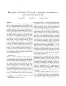
Figure 1: Different subgames in Quick Chess

Keywords Reinforcement Learning; Transfer Learning; Curriculum Learning

1.

INTRODUCTION

As autonomous agents are called upon to perform increasingly difficult tasks, new techniques will be needed to make learning such tasks tractable. Transfer learning [10, 27] is a recent area of research that has been shown to speed up learning on a complex task by transferring knowledge from one or more easier source tasks. However, most transfer learning methods assume the set of source tasks is provided, and treat the transfer of knowledge as a one-step process. Paradigms such as multi-task reinforcement learning and lifelong learning consider learning multiple tasks, but typically focus on optimizing performance over all tasks, and/or still require the set of tasks to be provided. In this paper, we extend transfer learning to the problem of curriculum learning. As a motivating example, conAppears in: Proceedings of the 15th International Conference on Autonomous Agents and Multiagent Systems (AAMAS 2016), J. Thangarajah, K. Tuyls, C. Jonker, S. Marsella (eds.), May 9–13, 2016, Singapore. c 2016, International Foundation for Autonomous Agents and Copyright Multiagent Systems (www.ifaamas.org). All rights reserved.

sider the game of Quick Chess1 (Figure 1). Quick Chess is a game designed to introduce players to the full game of chess, by using a sequence of progressively more difficult “subgames.” For example, the first subgame is a 5x5 board with only pawns, where the player learns how pawns move and about promotions. The second subgame is a small board with pawns and a king, which introduces a new objective: keeping the king alive. In each successive subgame, new elements are introduced (such as new pieces, a larger board, or different configurations) that require learning new skills and building upon knowledge learned in previous games. The final game is the full game of chess. The question that motivates us is: can we find an optimal sequence of subgames (i.e. a curriculum) for an agent to play that will make it possible to learn the target task of chess fastest, or at a performance level better than learning from scratch? We postulate that the effectiveness of such a curriculum depends crucially on the quality of the source tasks that compose it and the current learning abilities of the agent. As in Quick Chess, tasks should be designed to build upon existing knowledge and promote learning new skills. However, unlike Quick Chess, the tasks need not be the same for all agents. Thus, as a first step towards curriculum development, this paper focuses on how to automatically construct a space of useful subtasks. Our approach uses knowledge of the problem encoded via a parameterized model of the domain, and observes the agent’s performance on the target task and each prior task in the curriculum, in order to suggest new source tasks tailored to the abilities of the agent. Our three contributions are as follows. First, we introduce the problem of curriculum learning in the context of reinforcement learning (Section 3). Second, we propose a set of methods that can produce a space of agent-specific subtasks suitable for use in a curriculum (Section 4). Third, we 1 http://www.intplay.com/uploadedFiles/Game Rules/P20051QuickChess-Rules.pdf

566

experimentally show that training using a curriculum has a strong impact on the learning speed or performance of an agent, and that the sequence of tasks in the curriculum does matter. Furthermore, we demonstrate that the methods proposed can create such a curriculum, and be used successfully for transfer learning in Section 5. Section 6 compares our work with existing literature, and Section 7 concludes.

2.

The degrees of freedom F of a domain are a vector of features [F1 , F2 , . . . Fn ] that parameterize the domain. For example, in the Quick Chess domain, possible degrees of freedom could be the size of the board, the number of each type of piece, or whether special rules such as castling or en passant are allowed. Each Fi ∈ F has a range of values Rng(Fi ) that represents the possible values that feature can take. Furthermore, we assume there is an ordering defined over each Rng(Fi ) that corresponds to task complexity. Collectively, these degrees of freedom encode our domain knowledge in the task. An instantiation of F in D results in a specific task (an MDP). We assume we have a generator τ that can create tasks given a domain and degree of freedom vector:

BACKGROUND

We represent a task as an episodic Markov Decision Process (MDP) M . An MDP is a tuple (S, A, P, R, S0 , Sf ), where S is the set of states, A is the set of actions, P : S × A 7→ Π(S) is a transition function that gives the probability of moving to a new state given the current state and an action, and R : S × A 7→ R is a reward function that gives the immediate reward for taking an action in a state. S0 7→ Π(S) denotes the distribution over starting states, and Sf represents the set of terminal states. At each step, an RL agent observes its current state and chooses an action according to its policy π : S 7→ A. The goal of the agent is to learn an optimal policy π ∗ that maximizes the long-term expected sum of discounted rewards for some target task Mt . One standard way of doing this is to learn the optimal action-value function Q∗ (s, a), which gives the expected return for taking action a in state s and following policy π ∗ after: X Q∗ (s, a) = R(s, a) + P (s0 |s, a) max Q∗ (s0 , a0 ) 0 s0

τ : D × F 7→ M By restrictions, we mean the set of tasks that can be formed by eliminating certain actions or states, modifying the transition or reward function, or changing the starting or terminal distributions of MDPs generated by τ . Informally, D captures the universe of possible source tasks for use within the curriculum and could be potentially infinite in size. The goal of this paper is to create a subset of tasks in D that might be suitable for learning a given target task, using knowledge of the domain, and tailored to the performance and abilities of the learning agent. Formally, given a target task MDP Mt and trajectory samples X consisting of tuples (s, a, s0 , r) from following some policy πt on Mt , the goal is to create suitable source tasks Ms ∈ D that will lead to a policy in Mt that is better than πt . Specifically, we want functions f of the following form:

a

Q∗ is the unique solution to the Bellman equation above for all (s, a) pairs, and can be learned using methods such as Q-learning or Sarsa [22]. An optimal policy consists of choosing arg maxa Q∗ (s, a) in each state. In transfer learning, instead of learning directly on the target task Mt , the agent trains on one or more easier source tasks Ms , and transfers the knowledge acquired to the target task. This knowledge can take the form of samples [11, 12], options [21], policies [6], models [5], or value functions [26]. In this paper, we consider value function transfer, which uses the parameters of an action-value function Qs (s, a) learned in a source task to initialize the action-value function in the target task Qt (s, a). There are several metrics to quantify the benefit of transfer [27]. Typically, they compare the learning trajectory on the target task for an agent after transfer, with an agent that learns directly on the target task from scratch. In this work, we use asymptotic performance, which compares the final performance in the target task of learners when using transfer versus no transfer, and the jumpstart metric, which measures the initial performance increase on a target task as a result of transfer.

3.

f : Mt × X 7→ Ms The overall process we propose is an incremental development of subtasks culminating in a full curriculum: an agent first tries learning Mt , but gets stuck at suboptimal policy πt . X is generated from πt , and used to generate a space of possible source tasks tailored for this agent at this particular point in its learning process. For now, we assume a separate process is available to select a suitable source task Ms from this space, and leave for future work an automated way of finding it. The procedure then repeats, with Ms possibly becoming the new Mt , until a curriculum emerges.

4.

SEARCH SPACE FOR SOURCE TASKS

In this section, we describe several methods that can serve as f to create suitable source tasks for a target task. Intuitively, there are many different ways in which a task could be a useful source for transfer to Mt : it could have a smaller or more abstract state space; it could have some actions removed; it could focus on a useful subgoal; or it could drill a common mistake. Some of these source tasks could be generated by simply manipulating the degrees of freedom F , and indeed we consider that case first. However, in the rest of the section, we define additional domain-independent instantiations for f .

PROBLEM FORMULATION

In curriculum learning, the goal is to generate a sequence of source tasks M1 , M2 , . . . Mt for an agent to train on, such that the final asymptotic performance increases, or the learning time to reach a desired performance threshold decreases, versus following any other curriculum. As an important step towards this, we first define the domain D of possible tasks:

4.1

Task Dimension Simplification

The first method we propose, TaskSimplification (Algorithm 1), simplifies a task using knowledge of the domain’s parameterization. Here, Simplify is a function that changes one of the degrees of freedom Fi ∈ F to a new Fi0 ∈ Rng(Fi ),

Definition 1. A domain D is a set of MDPs that can be expressed by varying a set of degrees of freedom, and applying a set of restrictions.

567

in order to make the task smaller or easier. In many domains, there is a natural interpretation for Simplify. For example, in Quick Chess, we could reduce the value of parameters such as the size of the board or the number of specific pieces. In multiagent settings, we can add cooperative agents or remove adversarial ones.

action or sequence of actions (e.g., an option [23]) taken in a state that deviates from the optimal policy. In practice, the agent does not know the optimal policy while learning, so we propose 3 alternative characteristics to automatically identify mistakes. The first is any action that leads to unsuccessful termination of an episode, such as not reaching a goal state. Second is any action that results in no change in state. Finally, a mistake could be any action that incurs a large negative reward. In the following methods, we use IsMistake to denote whether a mistake was detected, using these criteria.

Algorithm 1 Task Simplification 1: procedure TaskSimplification(M, X, D, F, τ ) 2: F 0 = Simplify(F ) 3: M 0 ← τ (D, F 0 ) 4: return M 0 5: end procedure

Action Simplification The first mistake-driven subtask generation method we propose, ActionSimplification (Algorithm 3), prunes the action set to create a subtask where mistakes are less likely. Action set pruning is especially useful in settings where actions have preconditions for success. For example, a robot must grasp an object before manipulating it. An autonomous car must be standing still before opening the doors. Intuitively, any complex, multi-stage policy could benefit from this type of guided exploration.

TaskSimplification transforms the S, A, P, R elements of an MDP simultaneously, in a domain-specific way.

4.2

Promising Initializations

The second method is designed for tasks that have a sparse reward signal. In many RL problems, positive outcomes can be rare, especially at the onset of learning. An agent may have to reach the goal randomly or through some exploration scheme many times before the policy stabilizes. PromisingInitializations creates a task that initializes an agent near states that were found to have high reward.

Algorithm 3 Action Simplification 1: procedure ActionSimplification(M, X, α) 2: M0 ← M 3: count(a) = 0, ∀a ∈ A 4: Y ← {(s, a, s0 , r) ∈ X : IsMistake(s, a, s0 , r)} 5: for (s, a, s0 , r) ∈ Y do 6: count(a)+ = 1 7: end for 8: A0 = {a ∈ A : count(a) > α} 9: M 0 .A = M 0 .A \ A0 10: return M 0 11: end procedure

Algorithm 2 Promising Initializations 1: procedure PromisingInitializations(M, X, C, δ, ρ) 2: Y ← {(s, a, s0 , r) ∈ X : r ≥ ρth percentile of all rewards in X} 3: M0 ← M 4: S00 ← {} 5: for (s, a, s0 , r) ∈ Y do 6: S00 ← S00 ∪ FindNearbyStates(s, X, C, δ) 7: end for 8: M 0 .S0 ← S00 9: return M 0 10: end procedure

The parameter α ∈ Z is a threshold on the number of times an action should lead to a mistake before it is pruned. In practice, it may be useful to set these thresholds so that only one action is eliminated at a time, or only eliminated in certain states.

Here, the parameter ρ ∈ [0, 100] is a percentile that defines the fraction of rewards an agent has seen in its experience trajectory X that it should consider to be positive outcomes. FindNearbyStates is a domain-dependent function that returns a set/distribution of states that are close to a given state, using either a distance metric C : S × S 7→ R or a pseudo-distance based on steps away in a trajectory. The exact form depends on the representation used for the MDP. If the state space is factored, we can perturb the state vector by some amount δ such that the distance from the original state to the perturbed state (measured by C) is less than δ. In our Quick Chess example, if the state space consists of the positions of all pieces on the board, we can use a distance metric that measures the least number of “moves” needed to transform one board configuration to another. FindNearbyStates would return all configurations that are δ steps away. If the state space is not factored (for example, in a tabular representation), then we can use the trajectory samples X to find states that are at most δ steps away from a high reward state, and explore these further.

4.3

Mistake Learning In contrast, the second approach, MistakeLearning (Algorithm 4), directly tries to correct mistakes by rewinding the game back some number of steps, and having the agent learn a revised policy from there. Intuitively, focusing training on areas of the state space where the agent made a “mistake,” gives access to this experience much faster, allowing the agent to also learn to correct itself much faster. Algorithm 4 Mistake Learning 1: procedure MistakeLearning(M, X, ) 2: M0 ← M 3: S00 ← {} 4: Y ← {(s, a, s0 , r) ∈ X : IsMistake(s, a, s0 , r)} 5: for (s, a, s0 , r) ∈ Y do 6: S00 ← S00 ∪ Rewind(X, s, ) 7: end for 8: M 0 .S0 ← S00 9: return M 0 10: end procedure

Mistake-Driven Subtasks

Our next set of methods create subtasks to help an agent avoid and correct its mistakes. In principle, a mistake is any

568

The question of how far back in the trajectory to rewind is an interesting challenge in and of itself. For now, Rewind is a simple method that looks back  steps from s in trajectory X, and returns the found state. However, in principle it could be more complex, based on the type of mistake made or the situation where it was made. In our example of Quick Chess, we could rewind the game to determine what should have been done differently to avoid a checkmate.

4.4

ample, with a tabular representation, we can simply lookup states of high value. With function approximation, an optimization routine would be used to solve for high value states.

4.5

Task-based Subgoals

An alternative to creating subgoals within an MDP is to create them directly at the task level. Specifically, we set the termination set Sf of the input MDP to be the initiation set S0 of some other subtask, as shown in Algorithm 7:

Option-based Subgoals

Algorithm 7 Link Subtask 1: procedure LinkSubTask(M, Ms , V ) 2: M0 ← M 3: for s0 ∈ Ms .S0 , s ∈ M.S, a ∈ M.A do 4: R(s, a, s0 ) = V (s0 ) 5: end for 6: M 0 .Sf ← Ms .S0 7: M 0 .R ← R 8: return M 0 9: end procedure

The next method creates subtasks for learning subgoals. The options literature [23] identifies many approaches to finding subgoals. Many take a state-based approach, where the learner tries to find states that may have strategic value to reach. For example, McGovern and Barto [14], identify subgoals as states that occur frequently in successful trajectories. Menache et al. [15] try to find “bottleneck” states. Simsek and Barto [18] seek to create subgoals for “novel” states, since they facilitate exploration of regions of the state space that the agent normally doesn’t reach. Finally, graphbased approaches such as Mannor et al. [13] identify states by clustering over a state-transition map. OptionSubGoals (Algorithm 5) is designed to take any option discovery method (FindOption) to create a subtask. Specifically, it creates a task to learn an option given the option’s termination set Sf and a pseudo-reward function R for completion. Since an option typically only involves a subset of the task’s complete state space, this subtask allows quick learning of how to reach important states. For example, in Quick Chess, capturing the queen would be an example of a useful subgoal.

For example, we can create a subtask that terminates where PromisingInitializations starts as follows: M1 Ms

= =

PromisingInitializations(Mt , X, C, δ, ρ) LinkSubTask(Mt , M1 , M1 .V )

Applied to Quick Chess, this would create a task to reach configurations that are likely to lead to checkmate. The reward for reaching this terminal set is the value of the state in the subsequent task. This idea is similar to skill chaining [8], except that instead of learning options linking target regions to initiation sets, we link directly on tasks.

Algorithm 5 Option Sub-goals 1: procedure OptionSubGoals(M, X, V, φ) 2: M0 ← M 3: (Sf , R) ← FindOption(M, X, V, φ) 4: M 0 .Sf = Sf 5: M 0 .R = R 6: return M 0 7: end procedure

4.6

Composite Subtasks

Each of the previous subroutines f takes as input an MDP Mt and trajectory samples X, and returns a modified task MDP Ms . By passing the samples and resulting Ms as input to another function f , we can chain together arbitrary many subroutines to compose new source tasks. Mathematically, let f and g be any two functions above. Assume we are given a target task MDP Mt and trajectory samples X from it. Then, the composite task (f ◦ g) = f (g(Mt , X), X), where for ease of exposition, we’ve left out the task specific threshold parameters. Most of the domain-independent functions described previously make specific modifications to a particular part of the target task MDP. In contrast, TaskSimplification can potentially make changes to the state and action space, as well as the transition and reward functions all at once. Thus, in practice, tasks should be composed using TaskSimplification first, followed by the others.

Since our work takes place in the context of transfer learning, we introduce one additional option discovery method, FindHighValueStates (Algorithm 6), that uses high value states learned in a previous task as a subgoal. Specifically, it checks whether any of the learned values V (s) for states encountered in our trajectory X exceed a threshold φ. Algorithm 6 Find High Value States 1: procedure FindHighValueStates(M, X, V, φ) 2: Sf ← {} 3: R ← M.R 4: for (s, a, s0 , r) ∈ X do 5: if V (s) > φ then 6: Sf ← Sf ∪ s 7: R(s, a, s0 ) = V (s) 8: end if 9: end for 10: return (Sf , R) 11: end procedure

4.7

Summary

In summary, we presented several functions that could create suitable source tasks for a target task. They can be categorized into two types: the first (Section 4.1) allows for task creation using domain knowledge. The others are largely domain-independent, and rely directly on trajectory samples in the target task to create agent-specific tasks. We also showed how tasks of both types can be combined to create flexible source tasks for curriculum learning. We claim that the functions outlined are broadly and generally useful. However, they are not the only possible meth-

Instead of using trajectory samples X, we can also extract high value states directly from the value function. For ex-

569

Event Goal Ball out of bounds Ball with offense Ball captured by defense Ball captured by goalie Episode times out

ods; nor would every method apply to every domain. The next section moves on to experiments in domains for which we have concrete transfer learning results, using source tasks that can be generated with these functions.

5.

INSTANTIATIONS AND RESULTS

In this section, we apply the methods described in Section 4 to create a curriculum in two challenging multiagent domains: Ms. Pac-Man and Half Field Offense. First, we demonstrate the effectiveness of domain-dependent and domain-independent subtasks in a simple one-stage curriculum (i.e. classic transfer learning paradigm) applied to Ms. Pac-Man. Then, in Half Field Offense, we utilize multiple functions from Section 4 to create a successful multistage curriculum for learning. Furthermore, we show that the sequence of tasks in a curriculum matters, and provide empirical evidence that such curricula can be formed recursively.

5.1

Table 1: Reward structure in HFO This call creates a subtask that rewinds  = 50 game steps from the moment the episode was terminated. The agent subsequently trains for 5 episodes in the generated subtask, after which training in the target task is resumed. The result of this test is shown in Figure 4. For this experiment, we measured the agent’s performance as a function of the number of game steps, since episodes spent on learning in the generated subtasks were much shorter. Results are averaged over 20 trials. The plot shows that the application of MistakeLearning results in much faster learning when compared to the baseline approach of restarting each episode from the initial configuration upon episode termination. So far, the two examples show that both domain-dependent and domain-independent methods can be used to generate effective source tasks for a given target task. The next set of experiments demonstrate how, in addition, they can also be used to design a curriculum for an agent learning a task that may be too difficult to learn from scratch, or even using a single source task.

Ms. Pac-Man

Ms. Pac-Man (see Figure 2a and 2b) is a game where the agent’s goal is to traverse a maze and accrue points by eating objects such as pills, while avoiding the four ghosts. At the start of the game, there are a large number of pills throughout the maze, four power pills located at each corner, and four ghosts that are initially placed in an area inaccessible to Ms. Pac-Man. If a ghost catches Ms. Pac-Man, the game is over; however, if Ms. Pac-Man eats one of the four power pills, the ghosts themselves become edible by the agent. We used the Ms. Pac-Man implementation described in [24, 19]. The agent’s state space was represented by a set of local features described in [24], that are egocentric with respect to the agent’s position on the board. Learning was done using Q-Learning [22], and transfer via value function transfer.

5.1.1

5.2

Half Field Offense (HFO)

Half field offense [7] is a subtask of Robocup simulated soccer in which a team of m offensive players try to score a goal against n defensive players while playing on one half of a soccer field. The domain poses many challenges, including a large, continuous state and action space, coordination between multiple agents, and multiagent credit assignment. Each of these difficulties makes learning hard, especially early on when goal scoring episodes can be rare. Each HFO episode starts with the ball and offensive team placed randomly near the half field line. Likewise, the defensive team is randomly initialized near the goal box. A sample starting configuration can be seen in Figure 2c. The goal of the offensive team is to move the ball up the field while maintaining possession, and take shots to score on goal. An episode ends when either (1) a goal is scored, (2) the ball goes out of bounds, (3) the defense captures the ball, or (4) the episode times out. The reward structure of the domain is shown in Table 1. As done in Kalyanakrishnan et al. [7], we focus on learning behaviors for the player with the ball. The player with the ball has to choose one of the following actions:

Maze Simplification

The first experiment is an application of the TaskSimplification method. The domain of Ms. Pac-Man comes with four different maze levels, some of which are easier for the agent to learn than the others. Thus, intuitively, one way to apply the TaskSimplification method is to train an agent on an easier maze and transfer the learned policy to a harder one. The results of such an application are shown in Figure 3. Here, the target task was maze level four (Figure 2b). The TaskSimplification principle was used to generate a source task by changing the maze level from four to one (Figure 2a). The transfer curve shows the effects of learning for 5 episodes on the source task and then learning for an additional 20 episodes on the target task. The baseline curve in contrast shows the result of learning for 25 episodes directly on the target task. Both curves are averaged over 20 runs. The results clearly show that applying TaskSimplification results in jumpstart and substantial improvement in the expected reward over the first 25 episodes.

5.1.2

Reward 1.0 -0.1 0 -0.2 -0.1 -0.1

• Pass k: A direct pass to the teammate that is k-th closest to the ball, where k = 2, 3, . . . , m. • Dribble: A small kick in the cone formed between the player and the goalposts, that maximizes its distance to the closest defender also in the cone. • Shoot j: A full power kick towards one of j evenly spaced points on the goal line.

Avoiding Ghosts

Next, we illustrate the use of an agent-specific source task, MistakeLearning, in the Ms. Pac-Man domain. We consider a mistake to be the event where Ms. Pac-Man is eaten by a ghost, which is a terminal non-goal state. Whenever a mistake occurrs, we spawn the following task:

Offensive players without the ball follow one of several fixed formations to provide support. The agent’s state space

Mmistake = MistakeLearning(Mt , Xt , )

570

(a)

(b)

(c)

(d)

Figure 2: Examples of tasks in Ms. Pac-Man (a and b) and Half Field Offense (c and d). (a) Maze 1 (b) Maze 4 (c) HFO initial configuration and 2v2 dribble task (d) 2v2 shoot task. In HFO, offensive players are colored yellow, defensive players are blue, and the goalie is pink. The ball is shown by the white circle. 1400

2500

baseline transfer Expected Reward (points)

Expected Reward (points)

1200

1000

800

600

400

2000

1500

1000

500

200

baseline mistake learning 0

0 0

5

10

15

20

0

25

0.5

1

Game Steps

Episodes

1.5

2 5

x 10

Figure 3: Results of TaskSimplification applied to the Ms. Pac-Man domain. See Section 5.1.1 for details. Dashed lines indicate standard error.

Figure 4: Results of MistakeLearning applied to the Ms. Pac-Man domain. See Section 5.1.2 for details. Dashed lines indicate standard error.

consists of distances and angles to points of interest, which are listed in Table 2. We used CMAC tile coding for function approximation, Sarsa for the learning algorithm [22], and value function transfer to transfer knowledge.

For example, after observing generally unsuccessful trajectories on the target task, we could use MistakeLearning to recreate situations where the agent lost the ball or failed to score, in order to learn how to avoid or resolve them. Another option would be to build upon successful trajectories using PromisingInitializations, which would create tasks that initialize the offense at different positions near the goal, allowing them to drill on how to shoot. Combined, the methods from the previous section form a space of tasks that can be used to create a curriculum. In the next section, we illustrate the formal specification of some of the tasks and their creation that we found to be useful in our experiments.

Space of tasks Half field offense has a number of degrees of freedom that allow creating many different types of tasks. We list some of the relevant degrees of freedom in Table 3. In addition to these, various aspects of the field (such as the size of the goals, the goal box, etc.), the players (such as visibility, stamina, etc.), and the world physics can also be changed. These degrees of freedom allow us to quickly create many domain-specific source tasks, using the TaskSimplification rule. For example, we can add more teammates or reduce the number of defenders to give the offense more options. We can change the defensive team behavior to train against opponents of varying difficulty. We could also change various aspects of the world size and physics to make scoring and movement easier. However, we can also create agent-specific source tasks by observing the behavior of the agent on the target task.

5.2.1

2v2 HFO Curriculum

We first consider the target task of 2v2 half field offense, where 2 attackers must score against 1 defender and 1 goalie. We used agents from the released binaries of the Helios team to form the defensive team [1]. Helios and WrightEagle consistently place among the top teams in the annual Robocup 2D Simulation League tournament, making even this small version of half field offense a challenging task.

571

Feature dist-to-goalie dist-to-defender-incone dist-to-teammatei dist-teammatei -toclosest-defender dist-teammatei -passintercept min-ang-teammatei defender dist-to-shot-targeti dist-goalie-to-shottargeti dist-shoti -intercept

ang-goalie-shottargeti ang-defender-shottargeti

Description Distance from O1 to the goalie Distance from O1 to the closest defender in the dribble cone Distance from O1 to each teammate Oi , for i = 2, 3, . . . m For each Oi , the distance to its closest defender, i = 2, 3, . . . m For each Oi , the shortest distance between a defender and the line between O1 and Oi , i = 2, 3, . . . m For each Oi , the smallest angle between Oi , O1 , and a defender, i = 2, 3, . . . m Distance from O1 to location i on the goal line, i = 1, 2, . . . j Distance from goalie to location i on the goal line, i = 1, 2, . . . j Shortest distance between a defender and the line between O1 and location i on the goal line, i = 1, 2, . . . j Angle between goalie, O1 , and location i on the goal line, i = 1, 2, . . . j Smallest angle between a defender, O1 , and location i on the goal line, i = 1, 2, . . . j

ios are also possible to score from. We can gradually expand this set of states that lead to a high reward termination using PromisingInitializations, where we use a Euclidean distance metric C over the agent’s relative distances and angles to other players, to measure state proximity: Mshoot = PromisingInitializations(M2v2 , X2v2 , C, δ, ρ) A sample scenario can be seen in Figure 2d. Essentially, this task creates different configurations of players near the goal, and drills shooting. In our experiments, we set δ = 3 and ρ = 0.10.

Dribble Task Initially while exploring, the agent takes many shots on goal from far away, which are unlikely to score. A skill the agent needs is the ability to move the ball up the field, maintaining possession away from defenders, until the agent reaches a state that it can score from. This can be accomplished by chaining ActionSimplification with Mshoot using LinkSubTask: M1

=

LinkSubTask(M2v2 , Mshoot , Vshoot )

Mdribble

=

ActionSimplification(M1 , X2v2 , α)

LinkSubTask creates a subtask M1 where the goal is to reach situations that the agent is likely to score from, as learned in Mshoot . ActionSimplification prevents the agent from taking shots on goal from far away, since these actions usually lead to defense captures, and adds this restriction to M1 . An example of the initial configuration for the dribble task is shown in Figure 2c. In our experiments, we set α = 100.

Table 2: Feature space for the player with the ball in HFO. We index offensive players by their distance to the ball. Thus, the player with the ball is O1 and its teammates are O2 , O3 , . . . Om .

2v2 Curriculum Results Figure 5 shows the performance on the target task of 2v2 HFO for learners following various curricula composed of the 2 tasks above. For each curriculum, we trained on sub tasks until convergence. Offsets in the curves represent time spent training in source tasks. Labels indicate the curricula used; baseline is learning on the target task without transfer. The teams of agents were evaluated on their goal scoring ability: the fraction of times they are able to score a goal. Since each episode results in binary goal or no goal scored result, we used a sliding window of 200 episodes around each point to determine the average goal-scoring rate at each time step. All results are averaged over 25 trials. From Figure 5, it is clear to see that using a sequence of tasks to guide training significantly improves the final performance.

Let M2v2 denote the target task’s MDP, and X2v2 be a set of (presumably generally unsuccessful) samples collected from M2v2 . We can generate this task M2v2 = τ (D, F2v2 ), using the following instantiations for the degree of freedom vector (the order of parameters is the same as in Table 3): F2v2

=

[2, 2, Helios, flat, 68, 52.5, 2.7, 1, 0.3]

The following are specific subtasks that could be created using the methods from Section 4:

Shoot Task One useful skill to learn is where a goal can be scored from. After having obtained some experience in the target task with at least a few goals, it is very likely that similar scenar-

5.2.2 Parameter Number Offense Players Number Defense Players Defense Behavior Formation Type Field Width Field Length Max ball speed Max player speed Wind Noise

Range {0, 1, . . . 4} {0, 1, . . . 5} {Agent-2D, Helios, WrightEagle} { Flat, Box, Trapezoid} 20 – 68 20 – 52.5 0–5 0–1 0–1

Table 3: Half Field Offense degrees of freedom

Extension to 2v3 HFO

In this section, we extend the problem to the harder task of 2v3 half field offense, where there are now 2 defenders and a goalie. 2v3 is fundamentally harder than 2v2, since the additional defender means both attackers can now be marked. We can generate this target task M2v3 = τ (D, F2v3 ) using the following degree of freedom vector: F2v3 = [2, 3, Helios, flat, 68, 52.5, 2.7, 1, 0.3] This time, we can use TaskSimplification to simplify the degree of freedom vector to recreate the 2v2 task from the last section, allowing us to use it as a source for 2v3: M2v2 = TaskSimplification(M2v3 , X2v3 , D, F2v3 , τ )

572

Figure 5: Goal scoring accuracy on 2v2 HFO for agents following different curricula. Standard error (not shown to avoid clutter) ranged from 0.015 to 0.027 over the last 200 episodes for all curves.

Figure 6: Goal scoring accuracy on 2v3 HFO for agents following different curricula. Standard error (not shown to avoid clutter) ranged from 0.010 to 0.039 over the last 200 episodes for all curves.

Doing this also allows us to utilize the dribble and shoot tasks, since they are derived from M2v2 . Thus, we now consider 3 possible source tasks for a curriculum: Mdribble , Mshoot , and M2v2 . Results of various curricula composed of these source tasks can be seen in Figure 6. Again, using a multistage sequence of tasks provides better asymptotic performance than a curriculum composed of a subset of its source tasks. Interestingly, we also find that the most effective curriculum in 2v2 HFO is a subset of the best curriculum in 2v3 HFO when considering this space of tasks. This observation suggests that an automated procedure to create curricula could be designed recursively.

In fact, as far as we know, we are the first to propose general methods for creating source tasks for transfer learning. Past work has typically relied solely on domain knowledge to supply suitable source tasks. For example, 3v2 keepaway serving as a source for 4v3 keepaway [26], 2D mountain car as a source for 3D mountain car [25], or varying parameters of physical systems [2]. Sinapov et al. [19] use a set of task descriptors, which are similar to our degrees of freedom, to specify a set of source tasks. This work goes significantly beyond all of those by creating agent-specific tasks from a dynamic analysis of an agent’s performance, and shows how these tasks can be used in a multistage curriculum. Finally, the problem of source task selection, which is different from task generation has been considered in single step transfer learning as well [12, 19]. As before, they assume the set of tasks is already prespecified, and the goal is to select the best ones. Again, these tasks are not individualized for each agent, and thus depend on the quality of tasks present.

6.

RELATED WORK

Learning via a curriculum is an idea pervasive throughout human and animal training [20]. Recently, curriculum learning has also started to be explored in the context of supervised learning [3, 9], where the order in which individual samples are presented to an online learner was shown to considerably affect learning speed and generalization. Several related paradigms, such as multi-task learning [4] and lifelong learning [17], consider learning groups of prediction tasks. These methods assume tasks are related, and knowledge gained from solving one task can transfer to help learn another. In particular, Ruvolo and Eaton [16] show how a learner can actively select tasks to improve learning speed for all tasks, or for a specific target task. However, all of these works apply to supervised prediction tasks and assume the set of tasks to be learned is already given. Subsequently, many of these ideas have been studied in the reinforcement learning paradigm. For example, Wilson et al. [28] explored multi-task reinforcement learning while Ammar et al. [2] consider lifelong learning applied to sequential decision making tasks. In both cases, a sequence of RL tasks is presented to a learner, and the goal is to optimize over all tasks. In contrast, our source tasks are designed solely to improve performance on a target task. We aren’t concerned with optimizing performance in a source. In addition, neither work considers task generation, and thus are dependent on the quality of source tasks given.

7.

CONCLUSION

In this paper, we introduced the problem of curriculum learning in reinforcement learning. As a step towards this goal, we presented a series of functions that utilize domain knowledge and observations of an agent’s performance to create subtasks tailored to the agent. We showed how these subtasks could be used as components of a multistage curriculum to significantly improve an agent’s performance in two challenging multiagent reinforcement learning domains. A challenging next step in this research agenda is to develop automated methods for selecting from among the space of subtasks that our functions generate, in order to create a fully automated, individualized RL curriculum.

Acknowledgements This work took place in the Learning Agents Research Group (LARG) at UT Austin. LARG research is supported in part by NSF (CNS-1330072, CNS-1305287), ONR (21C184-01), AFRL (FA8750-14-1-0070), & AFOSR (FA9550-14-1-0087).

573

REFERENCES

[15] I. Menache, S. Mannor, and N. Shimkin. Q-cut dynamic discovery of sub-goals in reinforcement learning. In 13th European Conference on Machine Learning, pages 295–306. Springer, 2002. [16] P. Ruvolo and E. Eaton. Active task selection for lifelong machine learning. In Proceedings of the 27th AAAI Conference on Artificial Intelligence (AAAI-13), July 2013. [17] P. Ruvolo and E. Eaton. Ella: An efficient lifelong learning algorithm. In Proceedings of the 30th International Conference on Machine Learning (ICML-13), June 2013. [18] O. Simsek and A. G. Barto. Using relative novelty to identify useful temporal abstractions in reinforcement learning. In Proceedings of the Twenty-First International Conference on Machine Learning, pages 751–758, 2004. [19] J. Sinapov, S. Narvekar, M. Leonetti, and P. Stone. Learning inter-task transferability in the absence of target task samples. In Proceedings of the 2015 ACM Conference on Autonomous Agents and Multi-Agent Systems (AAMAS). ACM, 2015. [20] B. F. Skinner. Reinforcement today. American Psychologist, 13(3):94, 1958. [21] V. Soni and S. Singh. Using homomorphisms to transfer options across continuous reinforcement learning domains. In In Proceedings of American Association for Artificial Intelligence (AAAI), 2006. [22] R. Sutton and A. Barto. Reinforcement Learning: An Introduction. MIT Press, 1998. [23] R. Sutton, D. Precup, and S. Singh. Between mdps and semi-mdps: A framework for temporal abstraction in reinforcement learning. Artificial Intelligence, 112:181–211, 1999. [24] M. E. Taylor, N. Carboni, A. Fachantidis, I. Vlahavas, and L. Torrey. Reinforcement learning agents providing advice in complex video games. Connection Science, 26(1):45–63, 2014. [25] M. E. Taylor, G. Kuhlmann, and P. Stone. Autonomous transfer for reinforcement learning. In The Seventh International Joint Conference on Autonomous Agents and Multiagent Systems, May 2008. [26] M. E. Taylor and P. Stone. Behavior transfer for value-function-based reinforcement learning. In F. Dignum, V. Dignum, S. Koenig, S. Kraus, M. P. Singh, and M. Wooldridge, editors, The Fourth International Joint Conference on Autonomous Agents and Multiagent Systems, pages 53–59, New York, NY, July 2005. ACM Press. [27] M. E. Taylor and P. Stone. Transfer learning for reinforcement learning domains: A survey. Journal of Machine Learning Research, 10(1):1633–1685, 2009. [28] A. Wilson, A. Fern, S. Ray, and P. Tadepalli. Multi-task reinforcement learning: a hierarchical bayesian approach. In Proceedings of the 24th International Conference on Machine Learning, pages 1015–1022. ACM, 2007.

[1] H. Akiyama and T. Nakashima. HELIOS 2012: RoboCup 2012 Soccer Simulation 2D League Champion, volume 7500. Springer, 2012. [2] H. B. Ammar, E. Eaton, P. Ruvolo, and M. Taylor. Online multi-task learning for policy gradient methods. In Proceedings of the 31st International Conference on Machine Learning (ICML-14), pages 1206–1214, 2014. [3] Y. Bengio, J. Louradour, R. Collobert, and J. Weston. Curriculum learning. In Proceedings of the 26th Annual International Conference on Machine Learning, pages 41–48. ACM, 2009. [4] R. Caruana. Multitask learning. Machine learning, 28(1):41–75, 1997. [5] A. Fachantidis, I. Partalas, G. Tsoumakas, and I. Vlahavas. Transferring task models in reinforcement learning agents. Neurocomputing, 107:23–32, 2013. [6] F. Fern´ andez, J. Garc´ıa, and M. Veloso. Probabilistic policy reuse for inter-task transfer learning. Robotics and Autonomous Systems, 58(7):866 – 871, 2010. Advances in Autonomous Robots for Service and Entertainment. [7] S. Kalyanakrishnan, Y. Liu, and P. Stone. Half field offense in RoboCup soccer: A multiagent reinforcement learning case study. In RoboCup-2006: Robot Soccer World Cup X, volume 4434 of Lecture Notes in Artificial Intelligence, pages 72–85. Springer Verlag, Berlin, 2007. [8] G. Konidaris and A. Barto. Skill discovery in continuous reinforcement learning domains using skill chaining. In Advances in Neural Information Processing Systems, 2009. [9] M. P. Kumar, B. Packer, and D. Koller. Self-paced learning for latent variable models. In Advances in Neural Information Processing Systems, pages 1189–1197, 2010. [10] A. Lazaric. Transfer in reinforcement learning: a framework and a survey. In M. Wiering and M. van Otterlo, editors, Reinforcement Learning: State of the Art. Springer, 2011. [11] A. Lazaric and M. Restelli. Transfer from multiple MDPs. In Proceedings of the Twenty-Fifth Annual Conference on Neural Information Processing Systems (NIPS’11), 2011. [12] A. Lazaric, M. Restelli, and A. Bonarini. Transfer of samples in batch reinforcement learning. In A. McCallum and S. Roweis, editors, Proceedings of the Twenty-Fifth Annual International Conference on Machine Learning (ICML-2008), pages 544–551, Helsinki, Finalnd, July 2008. [13] S. Mannor, I. Menache, A. Hoze, and U. Klein. Dynamic abstraction in reinforcement learning via clustering. In Proceedings of the Twenty-First International Conference on Machine Learning, pages 560–567, 2004. [14] A. McGovern and A. G. Barto. Automatic discovery of subgoals in reinforcement learning using diverse density. In Proceedings of the Eighteenth International Conference on Machine Learning, pages 361–368, 2001.

574