SP2Bench: A SPARQL Performance Benchmark Michael Schmidt∗ ♯ , Thomas Hornung ♯ , Georg Lausen ♯ , Christoph Pinkel ♮ ♯
Freiburg University Georges-Koehler-Allee 51, 79110 Freiburg, Germany {mschmidt|hornungt|lausen}@informatik.uni-freiburg.de ♮
MTC Infomedia OHG Kaiserstrasse 26, 66121 Saarbr¨ucken, Germany
arXiv:0806.4627v2 [cs.DB] 21 Oct 2008
[email protected]
Abstract— Recently, the SPARQL query language for RDF has reached the W3C recommendation status. In response to this emerging standard, the database community is currently exploring efficient storage techniques for RDF data and evaluation strategies for SPARQL queries. A meaningful analysis and comparison of these approaches necessitates a comprehensive and universal benchmark platform. To this end, we have developed SP2 Bench, a publicly available, language-specific SPARQL performance benchmark. SP2 Bench is settled in the DBLP scenario and comprises both a data generator for creating arbitrarily large DBLP-like documents and a set of carefully designed benchmark queries. The generated documents mirror key characteristics and social-world distributions encountered in the original DBLP data set, while the queries implement meaningful requests on top of this data, covering a variety of SPARQL operator constellations and RDF access patterns. As a proof of concept, we apply SP2 Bench to existing engines and discuss their strengths and weaknesses that follow immediately from the benchmark results.
I. I NTRODUCTION The Resource Description Framework [1] (RDF) has become the standard format for encoding machine-readable information in the Semantic Web [2]. RDF databases can be represented by labeled directed graphs, where each edge connects a so-called subject node to an object node under label predicate. The intended semantics is that the object denotes the value of the subject’s property predicate. Supplementary to RDF, the W3C has recommended the declarative SPARQL [3] query language, which can be used to extract information from RDF graphs. SPARQL bases upon a powerful graph matching facility, allowing to bind variables to components in the input RDF graph. In addition, operators akin to relational joins, unions, left outer joins, selections, and projections can be combined to build more expressive queries. By now, several proposals for the efficient evaluation of SPARQL have been made. These approaches comprise a wide range of optimization techniques, including normal forms [4], graph pattern reordering based on selectivity estimations [5] (similar to relational join reordering), syntactic rewriting [6], specialized indices [7], [8] and storage schemes [9], [10], [11], [12], [13] for RDF, and Semantic Query Optimization [14]. Another viable option is the translation of SPARQL into SQL [15], [16] or Datalog [17], which facilitates the evaluation ∗ The
work of this author was funded by DFG grant GRK 806/2
with traditional engines, thus falling back on established optimization techniques implemented in conventional engines. As a proof of concept, most of these approaches have been evaluated experimentally either in user-defined scenarios, on top of the LUBM benchmark [18], or using the Barton Library benchmark [19]. We claim that none of these scenarios is adequate for testing SPARQL implementations in a general and comprehensive way: On the one hand, user-defined scenarios are typically designed to demonstrate very specific properties and, for this reason, lack generality. On the other hand, the Barton Library Benchmark is application-oriented, while LUBM was primarily designed to test the reasoning and inference mechanisms of Knowledge Base Systems. As a trade-off, in both benchmarks central SPARQL operators like O PTIONAL and U NION, or solution modifiers are not covered. With the SPARQL Performance Benchmark (SP2 Bench) we propose a language-specific benchmark framework specifically designed to test the most common SPARQL constructs, operator constellations, and a broad range of RDF data access patterns. The SP2 Bench data generator and benchmark queries are available for download in a ready-to-use format.1 In contrast to application-specific benchmarks, SP2 Bench aims at a comprehensive performance evaluation, rather than assessing the behavior of engines in an application-driven scenario. Consequently, it is not motivated by a single use case, but instead covers a broad range of challenges that SPARQL engines might face in different contexts. In this line, it allows to assess the generality of optimization approaches and to compare them in a universal, application-independent setting. We argue that, for these reasons, our benchmark provides excellent support for testing the performance of engines in a comprising way, which might help to improve the quality of future research in this area. We emphasize that such languagespecific benchmarks (e.g., XMark [20]) have found broad acceptance, in particular in the research community. It is quite evident that the domain of a language-specific benchmark should not only constitute a representative scenario that captures the philosophy behind the data format, but also leave room for challenging queries. With the choice of the DBLP [21] library we satisfy both desiderata. First, RDF has been particularly designed to encode metadata, which makes 1 http://dbis.informatik.uni-freiburg.de/index.php?project=SP2B
DBLP an excellent candidate. Furthermore, DBLP reflects interesting social-world distributions (cf. [22]), and hence captures the social network character of the Semantic Web, whose idea is to integrate a great many of small databases into a global semantic network. In this line, it facilitates the design of interesting queries on top of these distributions. Our data generator supports the creation of arbitrarily large DBLP-like models in RDF format, which mirror vital key characteristics and distributions of DBLP. Consequently, our framework combines the benefits of a data generator for creating arbitrarily large documents with interesting data that contains many real-world characteristics, i.e. mimics natural correlations between entities, such as power law distributions (found in the citation system or the distribution of papers among authors) and limited growth curves (e.g., the increasing number of venues and publications over time). For this reason our generator relies on an in-depth study of DBLP, which comprises the analysis of entities (e.g. articles and authors), their properties, frequency, and also their interaction. Complementary to the data generator, we have designed 17 meaningful queries that operate on top of the generated documents. They cover not only the most important SPARQL constructs and operator constellations, but also vary in their characteristics, such as complexity and result size. The detailed knowledge of data characteristics plays a crucial role in query design and makes it possible to predict the challenges that the queries impose on SPARQL engines. This, in turn, facilitates the interpretation of benchmark results. The key contributions of this paper are the following. 2 • We present SP Bench, a comprehensive benchmark for the SPARQL query language, comprising a data generator and a collection of 17 benchmark queries. • Our generator supports the creation of arbitrarily large DBLP documents in RDF format, reflecting key characteristics and social-world relations found in the original DBLP database. The generated documents cover various RDF constructs, such as blank nodes and containers. • The benchmark queries have been carefully designed to test a variety of operator constellations, data access patterns, and optimization strategies. In the exhaustive discussion of these queries we also highlight the specific challenges they impose on SPARQL engines. 2 • As a proof of concept, we apply SP Bench to selected SPARQL engines and discuss their strengths and weaknesses that follow from the benchmark results. This analysis confirms that our benchmark is well-suited to identify deficiencies in SPARQL implementations. • We finally propose performance metrics that capture different aspects of the evaluation process. Outline. We next discuss related work and design decisions in Section II. The analysis of DBLP in Section III forms the basis for our data generator in Section IV. Section V gives an introduction to SPARQL and describes the benchmark queries. The experiments in Section VI comprise a short evaluation of our generator and benchmark results for existing SPARQL engines. We conclude with some final remarks in Section VII.
II. B ENCHMARK D ESIGN D ECISIONS Benchmarking. The Benchmark Handbook [23] provides a summary of important database benchmarks. Probably the most “complete” benchmark suite for relational systems is TPC2 , which defines performance and correctness benchmarks for a large variety of scenarios. There also exists a broad range of benchmarks for other data models, such as object-oriented databases (e.g., OO7 [24]) and XML (e.g., XMark [20]). Coming along with its growing importance, different benchmarks for RDF have been developed. The Lehigh University Benchmark [18] (LUBM) was designed with focus on inference and reasoning capabilities of RDF engines. However, the SPARQL specification [3] disregards the semantics of RDF and RDFS [25], [26], i.e. does not involve automated reasoning on top of RDFS constructs such as subclass and subproperty relations. With this regard, LUBM does not constitute an adequate scenario for SPARQL performance evaluation. This is underlined by the fact that central SPARQL operators, such as U NION and O PTIONAL, are not addressed in LUBM. The Barton Library benchmark [19] queries implement a user browsing session through the RDF Barton online catalog. By design, the benchmark is application-oriented. All queries are encoded in SQL, assuming that the RDF data is stored in a relational DB. Due to missing language support for aggregation, most queries cannot be translated into SPARQL. On the other hand, central SPARQL features like left outer joins (the relational equivalent of SPARQL operator O PTIONAL) and solution modifiers are missing. In summary, the benchmark offers only limited support for testing native SPARQL engines. The application-oriented Berlin SPARQL Benchmark [27] (BSBM) tests the performance of SPARQL engines in a prototypical e-commerce scenario. BSBM is use-case driven and does not particularly address language-specific issues. With its focus, it is supplementary to the SP2 Bench framework. The RDF(S) data model benchmark in [28] focuses on structural properties of RDF Schemas. In [29] graph features of RDF Schemas are studied, showing that they typically exhibit power law distributions which constitute a valuable basis for synthetic schema generation. With their focus on schemas, both [28] and [29] are complementary to our work. A synthetic data generation approach for OWL based on test data is described in [30]. There, the focus is on rapidly generating large data sets from representative data of a fixed domain. Our data generation approach is more fine-grained, as we analyze the development of entities (e.g. articles) over time and reflect many characteristics found in social communities. Design Principles. In the Benchmark Handbook [23], four key requirements for domain specific benchmarks are postulated, i.e. it should be (1) relevant, thus testing typical operations within the specific domain, (2) portable, i.e. should be executable on different platforms, (3) scalable, e.g. it should be possible to run the benchmark on both small and very large data sets, and last but not least (4) it must be understandable. 2 See
http://www.tpc.org.
For a language-specific benchmark, the relevance requirement (1) suggests that queries implement realistic requests on top of the data. Thereby, the benchmark should not focus on correctness verification, but on common operator constellations that impose particular challenges. For instance, two SP2 Bench queries test negation, which (under closedworld assumption) can be expressed in SPARQL through a combination of operators O PTIONAL, F ILTER, and BOUND. Requirements (2) portability and (3) scalability bring along technical challenges concerning the implementation of the data generator. In response, our data generator is deterministic, platform independent, and accurate w.r.t. the desired size of generated documents. Moreover, it is very efficient and gets by with a constant amount of main memory, and hence supports the generation of arbitrarily large RDF documents. From the viewpoint of engine developers, a benchmark should give hints on deficiencies in design and implementation. This is where (4) understandability comes into play, i.e. it is important to keep queries simple and understandable. At the same time, they should leave room for diverse optimizations. In this regard, the queries are designed in such a way that they are amenable to a wide range of optimization strategies. DBLP. We settled SP2 Bench in the DBLP [21] scenario. The DBLP database contains bibliographic information about the field of Computer Science and, particularly, databases. In the context of semi-structured data one often distinguishes between data- and document-centric scenarios. Document-centric design typically involves large amounts of free-form text, while data-centric documents are more structured and usually processed by machines rather than humans. RDF has been specifically designed for encoding information in a machine-readable way, so it basically follows the datacentric approach. DBLP, which contains structured data and little free text, constitutes such a data-centric scenario. As discussed in the Introduction, our generator mirrors vital real-world distributions found in the original DBLP data. This constitutes an improvement over existing generators that create purely synthetic data, in particular in the context of a languagespecific benchmark. Ultimately, our generator might also be useful in other contexts, whenever large RDF test data is required. We point out that the DBLP-to-RDF translation of the original DBLP data in [31] provides only a fixed amount of data and, for this reason, is not sufficient for our purpose. We finally mention that sampling down large, existing data sets such as U.S. Census3 (about 1 billion triples) might be another reasonable option to obtain data with real-world characteristics. The disadvantage, however, is that sampling might destroy more complex distributions in the data, thus leading to unnatural and “corrupted” RDF graphs. In contrast, our decision to build a data generator from scratch allows us to customize the structure of the RDF data, which is in line with the idea of a comprehensive, language-specific benchmark. This way, we easily obtain documents that contain a rich set of RDF constructs, such as blank nodes or containers.
...
Fig. 1.
Extract of the DBLP DTD
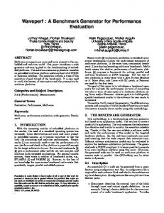
III. T HE DBLP DATA S ET The study of the DBLP data set in this section lays the foundations for our data generator. The analysis of frequency distributions in scientific production has first been discussed in [32], and characteristics of DBLP have been investigated in [22]. The latter work studies a subset of DBLP, restricting DBLP to publications in database venues. It is shown that (this subset of) DBLP reflects vital social relations, forming a “small world” on its own. Although this analysis forms valuable groundwork, our approach is of more pragmatic nature, as we approximate distributions by concrete functions. We use function families that naturally reflect the scenarios, e.g. logistics curves for modeling limited growth or power equations for power law distributions. All approximations have been done with the ZunZun4 data modeling tool and the gnuplot5 curve fitting module. Data extraction from the DBLP XML data was realized with the MonetDB/XQuery6 processor. An important objective of this section is also to provide insights into key characteristics of DBLP data. Although it is impossible to mirror all relations found in the original data, we work out a variety of interesting relationships, considering entities, their structure, or the citation system. The insights that we gain establish a deep understanding of the benchmark queries and their specific challenges. As an example, Q3a, Q3b, and Q3c (see Appendix) look similar, but pose different challenges based on the probability distribution of article properties discussed within this section; Q7, on the other hand, heavily depends on the DBLP citation system. Although the generated data is very similar to the original DBLP data for years up to the present, we can give no guarantees that our generated data goes hand in hand with the original DBLP data for future years. However, and this is much more important, even in the future the generated data will follow reasonable (and well-known) social-world distributions. We emphasize that the benchmark queries are designed to primarily operate on top of these relations and distributions, which makes them realistic, predictable and understandable. For instance, some queries operate on top of the citation system, which is mirrored by our generator. In contrast, the distribution of article release months is ignored, hence no query relies on this property. A. Structure of Document Classes Our starting point for the discussion is the DBLP DTD and the February 25, 2008 version of DBLP. An extract of 4 http://www.zunzun.com 5 http://www.gnuplot.info
3 http://www.rdfabout.com/demo/census/
6 http://monetdb.cwi.nl/XQuery/
the DTD is provided in Figure 1. The dblp element defines eight child entities, namely A RTICLE, I NPROCEEDINGS, . . ., and WWW resources. We call these entities document classes, and instances thereof documents. Furthermore, we distinguish between P ROCEEDINGS documents, called conferences, and instances of the remaining classes, called publications. The DTD defines 22 possible child tags, such as author or url, for each document class. They describe documents, and we call them attributes in the following. According to the DTD, each document might be described by arbitrary combination of attributes. Even repeated occurrences of the same attribute are allowed, e.g. a document might have several authors. However, in practice only a subset of all document class/attribute combinations occurs. For instance, (as one might expect) attribute pages is never associated with WWW documents, but typically associated with A RTICLE entities. In Table I we show, for selected document class/attribute pairs, the probability that the attribute describes a document of this class7 . To give an example, about 92.61% of all A RTICLE documents are described by the attribute pages. This probability distribution forms the basis for generating document class instances. Note that we simplify and assume that the presence of an attribute does not depend on the presence of other attributes, i.e. we ignore conditional probabilities. We will elaborate on this decision in Section VII. Repeated Attributes. A study of DBLP reveals that, in practice, only few attributes occur repeatedly within single documents. For the majority of them, the number of repeated occurrences is diminishing, so we restrict ourselves on the most frequent repeated attributes cite, editor, and author. Figure 2(a) exemplifies our analysis for attribute cite. It shows, for each documents with at least one cite occurrence, the probability (y-axis) that the document has exactly n cite attributes (x-axis). According to Table I, only a small fraction of documents are described by cite (e.g. 4.8% of all A RTICLE documents). This value should be close to 100% in real world, meaning that DBLP contains only a fraction of all citations. This is also why, in Figure 2(a), we consider only documents with at least one outgoing citation; when assigning citations later on, however, we first use the probability distribution of attributes in Table I to estimate the number of documents with at least one outgoing citation and afterwards apply the citation distribution in Figure 2(a). This way, we exactly mirror the distribution found in the original DBLP data. Based on experiments with different function families, we decided to use bell-shaped Gaussian curves for data approximation. Such functions are typically used to model normal distributions. Strictly speaking, our data is not normally distributed (i.e. there is the left limit x = 1), however, these curves nicely fit the data for x ≥ 1 (cf. Figure 2(a)). Gaussian curves are described by functions (µ,σ)
pgauss (x) =
x−µ 2 √1 e−0.5( σ ) , σ 2π
where µ ∈ R fixes the x-position of the peak and σ ∈ R>0 7 The
full correlation matrix can be found in Table IX in the Appendix.
TABLE I P ROBABILITY DISTRIBUTION FOR SELECTED ATTRIBUTES
author cite editor isbn journal month pages title
Article
Inproc.
Proc.
Book
WWW
0.9895 0.0048 0.0000 0.0000 0.9994 0.0065 0.9261 1.0000
0.9970 0.0104 0.0000 0.0000 0.0000 0.0000 0.9489 1.0000
0.0001 0.0001 0.7992 0.8592 0.0004 0.0001 0.0000 1.0000
0.8937 0.0079 0.1040 0.9294 0.0000 0.0008 0.0000 1.0000
0.9973 0.0000 0.0004 0.0000 0.0000 0.0000 0.0000 1.0000
specifies the statistical spread. For instance, the approximation function for the cite distribution in Figure 2(a) is defined by def (16.82,10.07) dcite (x) := pgauss (x). The analysis and the resulting distribution of repeated editor attributes is structurally similar def (2.15,1.18) and is described by the function deditor (x) := pgauss (x). The approximation function for repeated author attributes bases on a Gaussian curve, too. However, we observed that the average number of authors per publication has increased over the years. The same observation was made in [22] and explained by the increasing pressure to publish and the proliferation of new communication platforms. Due to the prominent role of authors, we decided to mimic this property. As a consequence, parameters µ and σ are not fixed (as it was the case for the distributions dcite and deditor ), but modeled as functions over time. More precisely, µ and σ are realized by limited growth functions8 (so-called logistic curves) that yield higher values for later years. The distribution is described by def
(µ
auth dauth (x, yr) := pgauss
def
µauth (yr) := def
σauth (yr) :=
(yr),σauth (yr))
2.05
(x), where
+ 1.05, and
1+17.59e−0.11(yr−1975) 1.00 + 1+6.46e−0.10(yr−1975)
0.50.
We will discuss the logistic curve function type in more detail in the following subsection. B. Key Characteristics of DBLP We next investigate the quantity of document class instances over time. We noticed that DBLP contains only few and incomplete information in its early years, and also found anomalies in the final years, mostly in form of lowered growth rates. It might be that, in the coming years, some more conferences for these years will be added belatedly (i.e. data might not yet be totally complete), so we restrict our discussion to DBLP data ranging from 1960 to 2005. Figure 2(b) plots the number of P ROCEEDINGS, J OURNAL, I NPROCEEDINGS, and A RTICLE documents as a function of time. The y-axis is in log scale. Note that J OURNAL is not an explicit document class, but implicitly defined by the journal attribute of A RTICLE documents. We observe that inproceedings and articles are closely coupled to the proceedings and journals. For instance, there are always about 50-60 times more 8 We make the reasonable assumption that the number of coauthors will eventually stabilize.
0.03
0.02
proceedings journals inproceedings articles approx. proceedings 10k approx. journals approx. inproceedings approx. articles
number of authors with publication count x
number of documents in year x
0.04 probability for x citations
100000
100k
probability for number of citations approx. probability for number of citations
1k
100
0.01
10
1
10
20 30 40 number of citations = x
50
Fig. 2.
60
1960
1970
1980 year = x
flogistic (x) =
a 1+be−cx ,
where a, b, c ∈ R>0 . For this parameter setting, a constitutes the upper asymptote and the x-axis forms the lower asymptote. The curve is “caught” in-between its asymptotes and increases continuously, i.e. it is S-shaped. The approximation function for the number of J OURNAL documents, which is also plotted in Figure 2(b), is defined by the formula def
2000
2005
10000
1000
100
10
1
5 10 publication count = x
50
80
(a) Distribution of citations, (b) Document class instances, and (c) Publication counts
inproceedings than proceedings, which indicates the average number of inproceedings per proceeding. Figure 2(b) shows exponential growth for all document classes, where the growth rate of J OURNAL and A RTICLE documents decreases in the final years. This suggests a limited growth scenario. Limited growth is typically modeled by logistic curves, which describe functions with a lower and an upper asymptote that either continuously increase or decrease for increasing x. We use curves of the form
fjournal (yr) :=
1990
in 1975 in 1985 in 1995 in 2005 approx. for 1975 approx. for 1985 approx. for 1995 approx. for 2005
740.43 . 1+426.28e−0.12(yr−1950)
Approximation functions for A RTICLE, P ROCEEDINGS, I N PROCEEDINGS , B OOK , and I NCOLLECTION documents differ only in the parameters. P H D T HESES, M ASTERS T HESES, and WWW documents were distributed unsteadily, so we modeled them by random functions. It is worth mentioning that the number of articles and inproceedings per year clearly dominates the number of instances of the remaining classes. The concrete formulas look as follows.
def
fdocs (yr) := fjournal (yr) + farticle (yr) + fproc (yr)+ finproc (yr) + fincoll + fbook (yr)+ fphd (yr) + fmasters (yr) + fwww (yr), The total number of authors, which we define as the number of author attributes in the data set, is computed as follows. First, we estimate the number of documents described by attribute author for each document class individually (using the distribution in Table I). All these counts are summed up, which gives an estimation for the total number of documents with one or more author attributes. Finally, this value is multiplied with the expected average number of authors per paper in the respective year (implicitly given by dauth in Section III-A). To be close to reality, we also consider the number of distinct persons that appear as authors (per year), called distinct authors, and the number of new authors in a given year, i.e. those persons that publish for the first time. We found that the number of distinct authors fdauth per year can be expressed in dependence of fauth as follows. def
fdauth (yr) := ( 1+169.41e−0.67 −0.07(yr−1936) + 0.84) ∗ fauth (yr) The equation above indicates that the number of distinct authors relative to the total authors decreases steadily, from 0.84% to 0.84%−0.67% = 0.17%. Among others, this reflects the increasing productivity of authors over time. The formula for the number fnew of new authors builds on the previous one and also builds upon a logistic curve: def
farticle (yr) fproc (yr) finproc (yr) fincoll (yr) fbook (yr) fphd (yr)
def
:=
def
:=
def
:=
def
:=
def
:=
def
58519.12 1+876.80e−0.12(yr−1950) 5502.31 1+1250.26e−0.14(yr−1965) 337132.34 1+1901.05e−0.15(yr−1965) 3577.31 196.49e−0.09(yr−1980) 52.97 40739.38e−0.32(yr−1950)
:= random[0..20]
def
fmasters (yr) := random[0..10] fwww (yr)
def
:= random[0..10]
C. Authors and Editors Based on the previous analysis, we can estimate the number of documents fdocs in yr by summing up the individual counts:
fnew (yr) := ( 1749.00e−0.29 −0.14(yr−1937) + 0.628) ∗ fdauth (yr) Publications. In Figure 2(c) we plot, for selected year and publication count x, the number of authors with exactly x publications in this year. The graph is in log-log scale. We observe a typical power law distribution, i.e. there are only a couple of authors having a large number of publications, while lots of authors have only few publications. Power law distributions are modeled by functions of the form fpowerlaw (x) = axk + b, with constants a ∈ R>0 , exponent k ∈ R 30min as used in our experiments here), Memory Exhaustion (if an additional memory limit was set), and general Errors. This metric gives a good survey over scaling properties and might give first insights into the behavior of engines. 2) L OADING T IME: The user should report on the loading times for the documents of different sizes. This metric primarily applies to engines with a database backend and might be ignored for in-memory engines, where loading is typically part of the evaluation process. 3) P ER -Q UERY P ERFORMANCE: The report should include the individual performance results for all queries over all document sizes. This metric is more detailed than the S UCCESS R ATE report and forms the basis for a deep study of the results, in order to identify strengths and weaknesses of the tested implementation. 4) G LOBAL P ERFORMANCE: We propose to combine the per-query results into a single performance measure. Here we recommend to list for execution times the arithmetic as well as the geometric mean, which is defined as the nth root of the product over n numbers. In the context of SP2 Bench, this means we multiply the execution time of all 17 queries (queries that failed should be ranked with 3600s, to penalize timeouts and other errors) and compute the 17th root of this product (for each document size, accordingly). This metric is well-suited to compare the performance of engines. 5) M EMORY C ONSUMPTION: In particular for engines with a physical backend, the user should also report on the high watermark of main memory consumption and ideally also the average memory consumption over all queries (cf. Table VI and VII). C. Benchmark Results for Selected Engines It is beyond the scope of this paper to provide an in-depth comparison of existing SPARQL engines. Rather than that, we use our metrics to give first insights into the state-of-the art and exemplarily illustrate that the benchmark indeed gives valuable hints on bottlenecks in current implementations. In this line, we are not primarily interested in concrete values (which, however, might be of great interest in the general case), but focus on the principal behavior and properties of engines, e.g. discuss how they scale with document size. We
will exemplarily discuss some interesting cases and refer the interested reader to the Appendix for the complete results. We conducted benchmarks for (1) the Java engine ARQ13 v2.2 on top of Jena 2.5.5, (2) the Redland14 RDF Processor v1.0.7 (written in C), using the Raptor Parser Toolkit v.1.4.16 and Rasqal Library v0.9.15, (3) SDB15 , which link ARQ to an SQL database back-end (i.e., we used mysql v5.0.34) , (4) the Java implementation Sesame16 v2.2beta2, and finally (5) OpenLink Virtuoso17 v5.0.6 (written in C). For Sesame we tested two configurations: SesameM , which processes queries in memory, and SesameDB , which stores data physically on disk, using the native Mulgara SAIL (v1.3beta1). We thus distinguish between the in-memory engines (ARQ, SesameM ) and engines with physical backend, namely (Redland, SBD, SesameDB , Virtuoso). The latter can further be divided into engines with a native RDF store (Redland, SesameDB , Virtuoso) and a relational database backend (SDB). For all physical-backend databases we created indices wherever possible (immediately after loading the documents) and consider loading and execution time separately (index creation time is included in the reported loading times). We performed three cold runs over all queries and documents of 10k, 50k, 250k, 1M , 5M , and 25M triples, i.e. inbetween each two runs we restarted the engines and cleared the database. We set a timeout of 30min (tme) per query and a memory limit of 2.6GB, either using ulimit or restricting the JVM (for higher limits, the initialization of the JVM failed). Negative and positive variation of the average (over the runs) was < 2% in almost all cases, so we omit error bars. For SDB and Virtuoso, which follow a client-server architecture, we monitored both processes and sum up these values. We verified all results by comparing the outputs, observing that SDB and Redland returned wrong results for a couple of queries, so we restrict ourselves on the discussion of the remaining four engines. Table IV shows the success rates. All queries that are not listed succeeded, except for ARQ and SesameM on the 25M document (either due to timeout or memory exhaustion) and Virtuoso on Q6 (due to missing standard compliance). Hence, Q4, Q5a, Q6, and Q7 are the most challenging queries, where we observe many timeouts even for small documents. Note that we did not succeed in loading the 25M triples document into the Virtuoso database. D. Discussion of Benchmark Results Main Memory. For the in-memory engines we observe that the high watermark of main memory consumption during query evaluation increases sublinearly to document size (cf. Table VI), e.g. for ARQ we measured an average (over runs and queries) of 85MB on 10k, 166MB on 50k, 318MB on 250k, 526MB on 1M , and 1.3GB on 5M triples. Somewhat 13 http://jena.sourceforge.net/ARQ/ 14 http://librdf.org/ 15 http://jena.sourceforge.net/SDB/ 16 http://www.openrdf.org/ 17 http://www.openlinksw.com/virtuoso/
TABLE IV S UCCESS RATES FOR QUERIES ON RDF DOCUMENTS UP TO 25M USE THE SHORTCUTS
TRIPLES . Q UERIES ARE ENCODED IN HEXADECIMAL ( E . G .,
’A’ STANDS FOR Q10). W E
+:=S UCCESS , T:=T IMEOUT, M:=M EMORY E XHAUSTION , AND E:=E RROR .
ARQ
SesameM
SesameDB
Virtuoso
Query
123 45 6789ABC abc ab
123 45 6789ABC abc ab
123 45 6789ABC abc ab
123 45 6789ABC abc ab
10k 50k 250k 1M 5M 25M
+++++++++++++++++ +++++++++++++++++ +++++T+++++++++++ +++++TT+TT+++++++ +++++TT+TT+++++++ TTTTTTTTTTTTTTTTT
+++++++++++++++++ +++++++++++++++++ ++++++T+T++++++++ ++++++T+TT+++++++ +++++TT+TT+++++++ MMMMMMMTMMMMMTMMT
+++++++++++++++++ +++++++++++++++++ ++++++T+TT+++++++ ++++++T+TT+++++++ +++++MT+TT+++++++ +++++TT+TT+++++++
++++++++E++++++++ ++++++++E++++++++ +++++TT+E++++++++ +++++TTTET+++++++ +++++TTTET+++++++ (loading of document failed)
TABLE V N UMBER OF
Query 10k 50k 250k 1M 5M 25M
QUERY RESULTS ON DOCUMENTS UP TO
25 MILLION TRIPLES
Q1
Q2
Q3a
Q3b
Q3c
Q4
Q5a
Q5b
Q6
Q7
Q8
Q9
Q10
Q11
1 1 1 1 1 1
147 965 6197 32770 248738 1876999
846 3647 15853 52676 192373 594890
9 25 127 379 1317 4075
0 0 0 0 0 0
23226 104746 542801 2586733 18362955 n/a
155 1085 6904 35241 210662 696681
155 1085 6904 35241 210662 696681
229 1769 12093 62795 417625 1945167
0 2 62 292 1200 5099
184 264 332 400 493 493
4 4 4 4 4 4
166 307 452 572 656 656
10 10 10 10 10 10
TABLE VI
TABLE VII
A RITHMETIC AND GEOMETRIC MEANS OF EXECUTION TIME (Ta /Tg ) AND ARITHMETIC MEAN OF MEMORY CONSUMPTION (Ma ) FOR THE
A RITHMETIC AND GEOMETRIC MEANS OF EXECUTION TIME (Ta /Tg ) AND ARITHMETIC MEAN OF MEMORY CONSUMPTION (Ma ) FOR THE NATIVE
IN - MEMORY ENGINES
ENGINES
ARQ
250k 1M 5M
SesameDB
SesameM
Ta [s]
Tg [s]
Ma [MB]
Ta [s]
Tg [s]
Ma [MB]
491.87 901.73 1154.80
56.35 179.42 671.41
318.25 525.61 1347.55
442.47 683.16 1059.03
28.64 106.38 506.14
272.27 561.79 1437.38
surprisingly, also the memory consumption of the native engines Virtuoso and SesameDB increased with document size. Arithmetic and Geometric Mean. For the in-memory engines we observe that SesameM is superior to ARQ regarding both means (see Table VI). For instance, the arithmetic (Ta ) and geometric (Tg ) mean for the engines on the 1M document over all queries18 are TaSesM = 683.16s, TgSesM = 106.84s, TaARQ = 901.73s, and TgARQ = 179.42s. For the native engines on 1M triples (cf. Table VII) we have TaSesDB = 653.17s, TgSesDB = 10.17s, TaV irt = 850.06s, and TgV irt = 3.03s. The arithmetic mean of SesameDB is superior, which is mainly due to the fact that it failed only on 4 (vs. 5) queries. The geometric mean moderates the impact of these outliers. Virtuoso shows a better overall performance for the success queries, so its geometric mean is superior. In-memory Engines. Figure 5 (top) plot selected results for in-memory engines. We start with Q5a and Q5b. Although both compute the same result, the engines perform much better for the explicit join in Q5b. We may suspect that the implicit join in Q5a is not recognized, i.e. that both engines compute 18 We
always penalize failure queries with 3600s.
250k 1M 5M
Virtuoso
Ta [s]
Tg [s]
Ma [MB]
Ta [s]
Tg [s]
Ma [MB]
639.86 653.17 860.33
6.79 10.17 22.91
73.92 145.97 196.33
546.31 850.06 870.16
1.31 3.03 8.96
377.60 888.72 1072.84
the cartesian product and apply the filter afterwards. Q6 and Q7 implement simple and double negation, respectively. Both engines show insufficient behavior. At the first glance, we might expect that Q7 (which involves double negation) is more complicated to evaluate, but we observe that SesameM scales even worse for Q6. We identify two possible explanations. First, Q7 “negates” documents with incoming citations, but – according to Section III-D – only a small fraction of papers has incoming citations at all. In contrast, Q6 negates arbitrary documents, i.e. a much larger set. Another reasonable cause might be the non-equality filter subexpression ?yr2 < ?yr inside the inner F ILTER of Q6. For A SK query Q12a both engines scale linearly with document size. However, from Table V and the fact that our data generator is incremental and deterministic, we know that a “witness” is already contained in the first 10k triples of the document. It might be located even without reading the whole document, so both evaluation strategies are suboptimal. Native Engines. The leftmost plot at the bottom of Figure 5 shows the loading times for the native engines SesameDB and Virtuoso. Both engines scale well concerning usr and sys, essentially linear to document size. For SesameDB , however,
ARQ (left) vs. SesameM (right)
usr+sys sys tme
10000 1000
Q5b ARQ (left) vs. SesameM (right)
usr+sys sys tme
10000
1000
Q6 ARQ (left) vs. SesameM (right)
usr+sys sys tme
10000
Q7 ARQ (left) vs. SesameM (right)
1000
1000
100
100
10
10
1
1
usr+sys sys tme
1000
1e+06 100000
Loading
10000 1000
S1 S2 S3 S4 S5 S6
0.1
S1 S2 S3 S4 S5 S6
S1 S2 S3 S4 S5 S6
0.01
Q2 SesameDB vs. Virtuoso (right)
1000
0.1
0.1
S1 S2 S3 S4 S5 S6
S1 S2 S3 S4 S5 S6
0.01
0.001
usr+sys sys tme
0.001
usr+sys sys tme
Q3a
100
SesameDB vs. Virtuoso (right)
1000
S1 S2 S3 S4 S5 S6
0.001
usr+sys sys tme
Q3c
10
SesameDB vs. Virtuoso (right)
usr+sys sys tme
Q10 SesameDB vs. Virtuoso (right)
10
100
S1 S2 S3 S4 S5 S6
0.01
100
10000 time in seconds
usr+sys sys tme
1
Failure Failure Failure
S1 S2 S3 S4 S5 S6
0.01 0.001
usr+sys sys tme SesameDB (left) vs. Virtuoso (right)
ARQ (left) vs. SesameM (right)
10
Failure Failure Failure
S1 S2 S3 S4 S5 S6
Failure
S1 S2 S3 S4 S5 S6
0.001
Failure
0.1
Failure Failure Failure Failure
0.1
Failure Failure Failure Failure
1
Failure Failure Failure
10
Failure Failure Failure
time in seconds
10
0.01
Q12a
100
100 100
1
10000
Failure
Q5a
Failure
10000
1
10
100
10
10
1
1 1
0.1 0.1
1
0.1
0.1
0.01
0.1
0.001
0.001 S1 S2 S3 S4 S5 S6
Fig. 5.
S1 S2 S3 S4 S5
0.01
0.01
0.01
0.01
0.001 S1 S2 S3 S4 S5 S6
S1 S2 S3 S4 S5
0.001 S1 S2 S3 S4 S5 S6
S1 S2 S3 S4 S5
0.001 S1 S2 S3 S4 S5 S6
S1 S2 S3 S4 S5
S1 S2 S3 S4 S5 S6
S1 S2 S3 S4 S5
Results for in-memory engines (top) and native engines (bottom) on S1=10k, S2=50k, S3=250k, S4=1M, S5=5M, and S6=25M triples
tme grows superlinearly (e.g., loading of the 25M document is about ten times slower than loading of the 5M document). This might cause problems for larger documents. The running times for Q2 increase superlinear for both engines (in particular for larger documents). This reflects the superlinear growth of inproceedings and the growing result size (cf. Tables VIII and V). What is interesting here is the significant difference between usr+sys and tme for Virtuoso, which indicates disproportional disk I/O. Since Sesame does not exhibit this peculiar behavior, it might be an interesting starting point for further optimizations in the Virtuoso engine. Queries Q3a and Q3c have been designed to test the intelligent choice of indices in the context of F ILTER expressions with varying selectivity. Virtuoso gets by with an economic consumption of usr and sys time for both queries, which suggests that it makes heavy use of indices. While this strategy pays off for Q3c, the elapsed time for Q3a is unreasonably high and we observe that SesameM scales better for this query. Q10 extracts subjects and predicates that are associated with Paul Erd¨os. First recall that, for each year up to 1996, Paul Erd¨os has exactly 10 publications and occurs twice as editor (cf. Section IV). Both engines answer this query in about constant time, which is possible due to the upper result size bound (cf. Table V). Regarding usr+sys, Virtuoso is even more efficient: These times are diminishing in all cases. Hence, this query constitutes an example for desired engine behavior. VII. C ONCLUSION We have presented the SP2 Bench performance benchmark for SPARQL, which constitutes the first methodical approach for testing the performance of SPARQL engines w.r.t. different operator constellations, RDF access paths, typical RDF constructs, and a variety of possible optimization approaches. Our data generator relies on a deep study of DBLP. Although it is not possible to mirror all correlations found in the original DBLP data (e.g., we simplified when assuming independence between attributes in Section III-A), many aspects
TABLE VIII C HARACTERISTICS OF GENERATED DOCUMENTS #Triples
10k
50k
250k
1M
5M
25M
file size [MB] data up to
1.0 1955
5.1 1967
26 1979
106 1989
533 2001
2694 2015
#Tot.Auth. #Dist.Auth.
1.5k 0.9k
6.8k 4.1k
34.5k 20.0k
151.0k 82.1k
898.0k 429.6k
5.4M 2.1M
#Journals #Articles #Proc. #Inproc. #Incoll. #Books #PhD Th. #Mast.Th. #WWWs
25 916 6 169 18 0 0 0 0
104 4.0k 37 1.4k 56 0 0 0 0
439 17.1k 213 9.2k 173 39 0 0 0
1.4k 56.9k 903 43.5k 442 356 101 50 35
4.6k 207.8k 4.7k 255.2k 1.4k 973 237 95 92
11.7k 642.8k 24.4k 1.5M 4.5k 1.7k 365 169 168
are modeled in faithful detail and the queries are designed in such a way that they build on exactly those aspects, which makes them realistic, understandable, and predictable. Even without knowledge about the internals of engines, we identified deficiencies and reasoned about suspected causes. We expect the benefit of our benchmark to be even higher for developers that are familiar with the engine internals. To give another proof of concept, in [33] we have successfully used SP2 Bench to identify previously unknown limitations of RDF storage schemes: Among others, we identified scenarios where the advanced vertical storage scheme from [12] was slower than a simple triple store approach. With the understandable DBLP scenario we clear the way for coming language modifications. For instance, SPARQL update and aggregation support are currently discussed as possible extensions.19 Updates, for instance, could be realized by minor extensions to our data generator. Concerning aggregations, the detailed knowledge of the document class counts and distributions (cf. Section III) facilitates the design of challenging aggregate queries with fixed characteristics. 19 See
http://esw.w3.org/topic/SPARQL/Extensions.
R EFERENCES [1] “Resource Description Framework (RDF): Concepts and Abstract Syntax,” http://www.w3.org/TR/rdf-concepts/. W3C Rec. 02/2004. [2] T. Berners-Lee, J. Hendler, and O. Lassila, “The Semantic Web,” Scientific American, May 2001. [3] “SPARQL Query Language for RDF,” http://www.w3.org/TR/rdfsparql-query/. W3C Rec. 01/2008. [4] J. Perez, M. Arenas, and C. Gutierrez, “Semantics and Complexity of SPAQRL,” in ISWC, 2006, pp. 30–43. [5] M. Stocker et al., “SPARQL Basic Graph Pattern Optimization Using Selectivity Estimation,” in WWW, 2008, pp. 595–604. [6] O. Hartwig and R. Heese, “The SPARQL Query Graph Model for Query Optimization,” in ESWC, 2007, pp. 564–578. [7] S. Groppe, J. Groppe, and V. Linnemann, “Using an Index of Precomputed Joins in order to speed up SPARQL Processing,” in ICEIS, 2007, pp. 13–20. [8] A. Harth and S. Decker, “Optimized Index Structures for Querying RDF from the Web,” in LA-WEB, 2005, pp. 71–80. [9] S. Alexaki et al., “On Storing Voluminous RDF descriptions: The case of Web Portal Catalogs,” in WebDB, 2001. [10] J. Broekstra, A. Kampman, and F. van Harmelen, “Sesame: A Generic Architecture for Storing and Querying RDF and RDF Schema,” in ISWC, 2002, pp. 54–68. [11] S. Harris and N. Gibbins, “3store: Efficient Bulk RDF Storage,” in PSSS, 2003. [12] D. J. Abadi et al., “Scalable Semantic Web Data Management Using Vertical Partitioning,” in VLDB, 2007, pp. 411–422. [13] C. Weiss, P. Karras, and A. Bernstein, “Hexastore: Sextuple Indexing for Semantic Web Data Management,” in VLDB, 2008. [14] G. Lausen, M. Meier, and M. Schmidt, “SPARQLing Constraints for RDF,” in EDBT, 2008, pp. 499–509. [15] R. Cyganiac, “A relational algebra for SPARQL,” HP Laboratories Bristol, Tech. Rep., 2005. [16] A. Chebotko et al., “Semantics Preserving SPARQL-to-SQL Query Translation for Optional Graph Patterns,” TR-DB-052006-CLJF. [17] A. Polleres, “From SPARQL to Rules (and back),” in WWW, 2007, pp. 787–796. [18] Z. P. Yuanbo Guo and J. Heflin, “LUBM: A Benchmark for OWL Knowledge Base Systems,” Web Semantics: Science, Services and Agents on the WWW, vol. 3, pp. 158–182, 2005. [19] D. J. Abadi et al., “Using the Barton libraries dataset as an RDF benchmark,” TR MIT-CSAIL-TR-2007-036, MIT. [20] A. Schmidt et al., “XMark: A Benchmark for XML Data Management,” in VLDB, 2002, pp. 974–985. [21] M. Ley, “DBLP Database,” http://www.informatik.uni-trier.de/∼ ley/db/. [22] E. Elmacioglu and D. Lee, “On Six Degrees of Separation in DBLP-DB and More,” SIGMOD Record, vol. 34, no. 2, pp. 33–40, 2005. [23] J. Gray, The Benchmark Handbook for Database and Transaction Systems. Morgan Kaufmann, 1993. [24] M. J. Carey, D. J. DeWitt, and J. F. Naughton, “The OO7 Benchmark,” in SIGMOD, 1993, pp. 12–21. [25] “RDF Vocabulary Description Language 1.0: RDF Schema,” http://www.w3.org/TR/rdf-schema/. W3C Rec. 02/2004. [26] “RDF Semantics,” http://www.w3.org/TR/rdf-mt/. W3C Rec. 02/2004. [27] C. Bizer and A. Schultz, “Benchmarking the Performance of Storage Systems that expose SPARQL Endpoints,” in SSWS, 2008. [28] A. Magkanaraki et al., “Benchmarking RDF Schemas for the Semantic Web,” in ISWC, 2002, p. 132. [29] Y. Theoharis et al., “On Graph Features of Semantic Web Schemas,” IEEE Trans. Knowl. Data Eng., vol. 20, no. 5, pp. 692–702, 2008. [30] S. Wang et al., “Rapid Benchmarking for Semantic Web Knowledge Base Systems,” in ISWC, 2005, pp. 758–772. [31] C. Bizer and R. Cyganiak, “D2R Server publishing the DBLP Bibliography Database,” 2007, http://www4.wiwiss.fu-berlin.de/dblp/. [32] A. J. Lotka, “The Frequency Distribution of Scientific Production,” Acad. Sci., vol. 16, pp. 317–323, 1926. [33] M. Schmidt et al., “An Experimental Comparison of RDF Data Management Approaches in a SPAQL Benchmark Scenario,” in ISWC, 2008.
A PPENDIX SELECT ?yr Q1 WHERE { ?journal rdf:type bench:Journal. ?journal dc:title "Journal 1 (1940)"ˆˆxsd:string. ?journal dcterms:issued ?yr } SELECT ?inproc ?author ?booktitle ?title Q2 ?proc ?ee ?page ?url ?yr ?abstract WHERE { ?inproc rdf:type bench:Inproceedings. ?inproc dc:creator ?author. ?inproc bench:booktitle ?booktitle. ?inproc dc:title ?title. ?inproc dcterms:partOf ?proc. ?inproc rdfs:seeAlso ?ee. ?inproc swrc:pages ?page. ?inproc foaf:homepage ?url. ?inproc dcterms:issued ?yr OPTIONAL { ?inproc bench:abstract ?abstract } } ORDER BY ?yr (a) SELECT ?article Q3 WHERE { ?article rdf:type bench:Article. ?article ?property ?value FILTER (?property=swrc:pages) } (b) Q3a, but "swrc:month" instead of "swrc:pages" (c) Q3a, but "swrc:isbn" instead of "swrc:pages" SELECT DISTINCT ?name1 ?name2 WHERE { ?article1 rdf:type bench:Article. ?article2 rdf:type bench:Article. ?article1 dc:creator ?author1. ?author1 foaf:name ?name1. ?article2 dc:creator ?author2. ?author2 foaf:name ?name2. ?article1 swrc:journal ?journal. ?article2 swrc:journal ?journal FILTER (?name1