1
Space-Optimal, Wait-Free Real-Time Synchronization Hyeonjoong Cho, Binoy Ravindran
E. Douglas Jensen
ECE Dept., Virginia Tech
The MITRE Corporation
Blacksburg, VA 24061, USA
Bedford, MA 01730, USA
{hjcho,binoy}@vt.edu
[email protected]
Abstract We consider wait-free synchronization for the single-writer/multiple-reader problem in small-memory embedded real-time systems. We present an analytical solution to the problem of determining the minimum, optimal space cost required for this problem, considering a-priori knowledge of interferences — the first such result. We also show that the space costs required by previous algorithms can be obtained by our analytical solution, which subsumes them as special cases. We also present a waitfree protocol that utilizes the minimum space cost determined by our analytical solution. Our evaluation studies and implementation measurements using the SHaRK RTOS kernel validate our analytical results.
I. I NTRODUCTION Most embedded real-time systems involve mutually exclusive, concurrent access to shared data objects, resulting in contention for those objects. Resolution of the contention directly affects the system’s timeliness, and thus the system’s behavior. Mechanisms that resolve such contention can be broadly classified into: (1) lock-based—e.g., Priority Inheritance and Ceiling protocols [1], Stack Resource Policy [2], DASA [3]; (2) wait-free—e.g., NBW protocol [4], Chen’s protocol [5], [6], [7]; and (3) lock-free—e.g., [8].
2
Lock-based protocols have several disadvantages such as serialized access to shared objects, resulting in reduced concurrency and thus reduced resource utilization [8]. Further, many lockbased protocols typically incur additional run-time overhead due to increased context switching between activities blocked on shared objects (i.e., “blockers”) and activities that hold locks of those objects (i.e., “lock holders”). The increased context switching occurs when lock-based protocols preempt the currently executing blocker, execute the lock holder until the holder releases the lock, and then resume the blocker’s execution. Another disadvantage of using locks is the possibility of deadlocks that can occur when lock holders crash, causing indefinite starvation to blockers. Further, many (real-time) lock-based protocols require a-priori knowledge of the ceilings of the locks [1], [2], which may be difficult to obtain in some application contexts. Furthermore, OS data structures (e.g., semaphore control blocks) must be a-priori updated with that knowledge, resulting in reduced flexibility (e.g., recompilation to accommodate new activities) [8]. These drawbacks have motivated research on wait-free and lock-free object sharing in realtime systems. Wait-free protocols use multiple internal buffers1 (e.g., a circular buffer) for writers and readers [4]. For the single-writer/multiple-reader (or SWMR) problem, wait-free protocols typically use multiple buffers for the shared object, where the number of buffers used is proportional to the maximum number of times the readers can be interfered by the writer, when the readers are reading. The maximum number of interferences of a reader bounds the number of times the writer can update the object while the reader is reading. Thus, by using as many buffers as the worst-case number of interferences of readers, the readers and the writer 1
We use the term internal here to explicitly indicate that a single wait-free buffer internally uses multiple buffers for its atomic
operations. In this paper, the buffers and the space cost implicitly mean the internal buffers and the cost of the internal buffers, respectively, unless otherwise noted.
3
can continuously read and write in different buffers, respectively, and avoid interference. Lock-free protocols allow readers to concurrently read while the writer is writing (without acquiring locks), but the readers check whether their reading was interfered by the writer. If so, they read again. Thus, a reader continuously reads, checks, and retries until its read becomes successful. Since a reader’s worst-case number of retries depends upon the worst-case number of times the reader is interfered by the writer, the additional execution-time overhead incurred for the retries is bounded by the number of interferences. Both wait-free and lock-free protocols incur additional costs with respect to their lock-based counterparts. Wait-free protocols generally incur additional space costs due to their multiple buffer usage, which is infeasible in many small-memory, embedded real-time systems. Lockfree protocols generally incur additional time costs due to their retries, which is antagonistic to timeliness optimization. Prior research have shown how to mitigate these space and time costs, so that they are feasible for embedded real-time systems. An excellent survey of this prior research can be found in [7]. To provide context for our work, we summarize some important efforts here: In [4], Kopetz and Reisinger present one of the earliest wait-free protocols, where buffer sizes in proportional to worst-case interferences are used. In [8], Anderson et al. show how to bound the retry loops of lock-free protocols through judicious scheduling. In [5], Chen and Burns present one of the most space-efficient wait-free protocols, where the worst-case preemptions need not be a-priori known. In [9], Sundell and Tsigas describe a wait-free protocol for the multiple-writer/multiple-reader problem. In [7], Huang et al. improve the time and space costs of Chen’s protocol. In this paper, we focus on wait-free synchronization for the SWMR problem in small-memory, embedded real-time systems. We focus on wait-free, as opposed to lock-free, as majority of the lock-free protocols have high computational costs [7]. We consider the SWMR problem, as it
4
occurs in most embedded real-time systems [7], and focus on minimizing its space costs. We present an analytical solution to the problem of determining the minimum number of buffers that is required to ensure the safety and orderliness of wait-free synchronization in SWMR. We call this problem, Wait-Free Buffer size decision Problem (or WFBP). Note that the optimality in space that we provide is on the required number of internal buffers, and does not include the control variables needed for the wait-free protocol’s operation. This is because the space cost of internal buffers dominates that of the control variables, especially when the data size becomes larger. We prove that our solution to WFBP subsumes the number of buffers required by previous wait-free protocols including Chen’s [5] and NBW [4] protocols as special cases. We analytically identify the conditions under which our protocol needs less (and equal) number of buffers than other protocols. Further, we present a wait-free protocol that utilizes the minimum buffer requirement determined by our solution. To determine the buffer requirements under a broad range of reader/writer scenarios, we conduct numerical evaluations. We also implement our protocol in the SHaRK RTOS [10]. Our evaluations and implementation measurements confirm our solution to WFBP and validate our analytical results. Thus, the paper’s contributions include the analytical solution that we present for WFBP and the wait-free protocol that uses the concomitant minimum number of buffers. Among the class of wait-free protocols that consider a-priori knowledge of interferences, our optimal space lower bound is the first such bound that is analytically established. The rest of the paper is organized as follows: We present our analytical solution to WFBP and our wait-free protocol in Section II. In Section III, we formally compare our protocol with Chen’s and NBW protocols. We numerically evaluate our protocol in Section IV, and report our implementation experience in Section V. We conclude the paper in Section VI.
5
II. A S PACE -O PTIMAL WAIT-F REE P ROTOCOL A wait-free protocol solves the asynchronous single-writer/multiple-reader problem by ensuring that each reader accesses the shared object without any interference from the writer. To realize the wait-free mechanism, the protocol must hold two properties: safety and orderliness [5]. The safety property ensures that the shared object does not become corrupted during reading and writing. The orderliness property ensures that all readers always read the latest data that is completely written by the writer. The basic idea to achieve the two properties is rooted in the three-slot fully asynchronous mechanism for the single-reader/single-writer problem [11]. For this problem, Chen et al. show that three buffers are required to keep the latest completely updated buffer for the next reading, while a writer and a reader are occupying buffers respectively. This mechanism allows that a reader can always obtain data from the buffer slot that is last completely updated, while the writer is writing the new version of the shared data [5]. The buffers needed for the single-writer/multiple-reader problem consist of three types: buffers for readers, a buffer for the latest written data, and a buffer for the next write operation. The buffers for readers must satisfy safety—i.e., sufficient buffers must be available to avoid interference between reading and writing. However, this does not imply that we need as many buffers as there are readers. The two buffers for writing are required to realize orderliness—i.e., the latest written data must be saved so that a newly activated reader can access it at any time. In addition, the latest written data must be kept until the writer completely writes the next data into another buffer. We now discuss how to determine the minimum number of buffers that are needed for the single-writer/multiple-reader problem in the following subsections:
6
A. Protocol Structure and Task Model Figure 1 shows a wait-free protocol’s common implementation. W.2 and R.2 show the code sections of the writer and a reader that write and read data, respectively. W.1 is the code section where the writer decides on the buffer for writing, and updates a control variable that indicates the selected buffer. W.3 is the code section where the writer indicates completion of writing and the buffer that has the latest data. In R.1, the reader checks for the latest data to read.
(a) Write Fig. 1.
(b) Read
Typical Wait-Free Implementation
The buffer size required for the NBW protocol [4] and the improved protocols in [7] is determined based on the temporal properties of tasks. These prior works consider the periodic task model, where tasks concurrently share data objects. Aperiodic tasks are handled by a periodic server, so the periodic model is not a limiting assumption. Assuming that all deadlines are met (i.e., during under-load situations and precluding overloads), the maximum number of preemptions of the reader by the writer task in the worst-case can be obtained. We consider the same task model.
B. Number of Buffers in Use We introduce some notations for convenience, most of which are similar to those in [5]. We denote the total number of readers as M and the ith reader as Ri . The reader Ri ’s j th instance
7 [j]
of reading is denoted as Ri . The writer’s k th writing instance is denoted as W [k] . [j]
[j]
[j]
Ri (op) stands for a specific operation of Ri . For example, Ri (READIN G[i] = 0) implies the execution of one statement in Chen’s algorithm [5]. W [k] (op) also stands for the operation [j]
[j]
in W [k] . If Ri reads what W [k] writes, we denote it as w(Ri ) = W [k] . As previously mentioned, safety and orderliness can be achieved with multiple buffers for readers, one buffer for the latest written data, and another buffer for the next writing.
Fig. 2.
Number of Buffers in Use
Suppose we have 4 readers and 1 writer, as shown in Figure 2. At time t1 , w(R1 )=W [2] , w(R2 )=W [2] , and w(R3 )=W [1] . This implies that two buffers are being used by the readers. In addition, one buffer is required to store and save the latest completely written data by W [4] , and another is needed for the next writing operation by W [5] . Thus, four buffers are being used in total, at time t1 . At time t2 , w(R1 )=W [6] , w(R2 )=W [5] , w(R3 )=W [4] , and w(R4 )=W [6] . The latest written data is by W [6] , and W [7] is the next operation. Thus, the total number of buffers used at time t2 is four, which is the minimum number required at t2 for ensuring safety and orderliness properties. The basic intuition for determining the minimum number of buffers is to construct a worstcase where the required number of buffers is as large as possible, when the maximum possible number of interferences of all readers with the writer occurs. We map this problem to a problem
8
called the Diverse Selection Problem (or DSP) and then solve it.
C. Diverse Selection Problem ~ x)) is defined with the problem range R and the range vector The DSP denoted as D(R, R(~ ~ x) of all elements in the vector ~x. R has the lower and upper bounds defined as [l, u]. Each R(~ element xi in the vector ~x has the range ri =[li , ui ]. The solution to the problem D is represented as a vector ~x =< x1 , ..., xM > where the vector size n(~x) is M . Every xi must satisfy its range constraint ri and the problem range constraint R. We define {~x} as a set including all elements of ~x, but without duplicates. Thus, the size of {~x}, n({~x}), is less than or equal to n(~x). The objective of DSP is to determine the maximum n({~x}) by selecting ~x, satisfying all range constraints as diversely as possible. Given a vector, ~v =< v1 , ..., vi , ... >, we denote the number of vi ’s having k value as H(~v , k), ~ ~x ), the optimal solution and the maximum value among all vi elements as T op(~v ). Given D(R, R of D when R = [t1 , t2 ] is denoted as nmax x}). [t1 ,t2 ] ({~ For example, if ~v =< 1, 2, 2, 2, 6 > then, H(~v , 2) = 3 and T op(~v ) = 6. An easy approach to solve DSP is by considering all possible cases. The number of all possible cases is n(r1 ) × ... × ~ of the problem is given as < r1 , ...rM >. By considering all cases, we can n(rM ), where the R select a vector ~x that maximizes n({~x}). However, such an approach would be computationally expensive. A more efficient approach to solve DSP can be found by an inductive strategy. Consider ~ x)), where R = [1, ∞] and R=< ~ a DSP D(R, R(~ [1, u1 ], ..., [1, uM ] >. If all lower bounds of ~ for elements of ~x are 1, we can define the upper bound vector ~u =< u1 , ..., uM > instead of R, convenience. In the rest of the paper, we call the problem defined by D(R, ~u) as DSP. This is simply because this assumption is well-mapped to the problem of deciding the minimum buffer
9
size for the wait-free protocol.
Fig. 3.
An Inductive Approach to DSP
The solution to the problem D(R, ~u) can be represented as nmax x}). The idea to [1,T op(~ u)] ({~ decompose the problem is shown in Figure 3. If the solution to the problem D([6, 12], ~u) can be derived from the solution to the problem D([7, 12], ~u), we can inductively determine the final solution to the problem D([1, 12], ~u). Theorem 2.1 (DSP for the Wait-Free Protocol): In the DSP D(R, ~u) with R = [1, N ], P nmax x}) + 1, if t+1 u, N − k) > nmax x}) k=0 H(~ [t] ({~ [t] ({~ max n[t+1] ({~x}) = max n ({~x}), otherwise [t]
where N = T op(~u), [t]=[N − t, N ], and 0 ≤ t < N . When t = 0, the nmax x}) = 1. [0] ({~ Proof: Assume that we have the solution to the problem D([N − t, N ], ~u). When this problem is extended to D([N − (t + 1), N ], ~u), the ranges of several variables xi overlap with the problem range [N − (t + 1), N ]. The number of newly added variables that we need to consider is H(~u, N − (t + 1)). When the problem range is extended by 1, the maximum possible increment of nmax x}) is 1. The increment happens only if the number of all xi which have [t+1] ({~
10
their ri overlapped with [N − (t + 1), N ] is greater than nmax x}). In other words, this happens [t] ({~ when new elements appear in the extended problem scope, or there is an element duplicated x}) has no change from before. The within [N − t, N ] at the previous step. Otherwise, nmax [t+1] ({~ increment means that the value of one element is determined as diversely as possible. The proof is by induction on t. Basis. We show that the theorem holds when t = 0. When the problem is D([T op(~u), T op(~u)], ~u), there must be at least one element xi with the range [1, T op(~u)], and the maximum possible value of nmax x}) is 1. Hence, the basis for the induction holds. [0] ({~ Induction step. Assume that the theorem holds true when R = [N − t, N ]. We arrive at the optimal solution of D([N − (t + 1), N ], ~u) with the optimal solution of D([N − t, N ], ~u) as in the base step. Suppose that the derived solution nmax x}) is not optimal. Then, there must [t+1] ({~ exist another optimal solution nmax x}0 ). Clearly, nmax x}0 ) is greater than nmax x}). Now, [t+1] ({~ [t+1] ({~ [t+1] ({~ there are two possible cases: Case 1. If H(~u, N − (t + 1)) > nmax x}), then nmax x}) is nmax x}) + 1, which is less [t] ({~ [t+1] ({~ [t] ({~ than nmax x}0 ). Therefore, nmax x}) < nmax x}0 ) − 1. This means that there exists another [t+1] ({~ [t] ({~ [t+1] ({~ {~x} that has more than nmax x}) elements. This contradicts the assumption that nmax x}) is [t] ({~ [t] ({~ optimal. Case 2. If H(~u, N − (t + 1)) = n[t] ({~x}), then nmax x}) is nmax x}), which is less [t+1] ({~ [t] ({~ than nmax x}0 ). Since no element’s range becomes newly overlapped and no element has its [t+1] ({~ duplicate, nmax x}0 ) = nmax x}0 ). This means that there exists another nmax x}0 ), which is [t+1] ({~ [t] ({~ [t] ({~ greater than nmax x}). This contradicts the assumption that nmax x}) is optimal. [t] ({~ [t] ({~ Theorem 2.2 (Solution Vector for the DSP): In the DSP D(R, ~u) with R = [1, N ], P {~ x}[t] ∪ {N − (t + 1)}, if t+1 u, N − k) > nmax x}), k=0 H(~ [t] ({~ {~x}[t+1] = {~ x}[t] , otherwise
11
where N = T op(~u), [t]=[N − t, N ], and 0 ≤ t < N . When t = 0, {~x}[0] = {N }. Proof: By Theorem 2.1, {~x} can be constructed by adding {N − (t + 1)} whenever nmax ({~x}) increases by 1. Note that this {~x} is one of the solution vectors. t
D. Similarity to WFBP The DSP has similarity with the Wait-Free Buffer size decision Problem (or WFBP). In this max problem, we are given M readers and their maximum interferences as < N1max , ..., NM >. The
objective of WFBP is to determine the worst-case maximum number of buffers.
Fig. 4.
A Worst-Case of the WFBP
Figure 4 illustrates how to construct the worst-case where the required number of buffers are as large as possible with an example. For convenience, the index of the writer is reversed compared with Figure 2. In this example, R1 ’s maximum interference is 5, which is illustrated in a line. It means that w(R1 ) may belong to the set {W [1] ,...,W [6] }. We assume that the worst-case happens at time t between W [2] and W [1] , where W [2] writes the latest completely written data, and W [1] is the next writing operation for which another buffer is needed. For this reason, we restate WFBP as determining ~x =< w(R1 ), ..., w(RM ) > that will max +1]
maximize n({~x}∪{W [1] , W [2] }), where w(Ri ) ∈ {W [1] , ..., W [Ni
}. If we abbreviate W [j] as
j, the problem is redefined as determining ~x =< x1 , ..., xM > that will maximize n({~x}∪{1, 2}),
12
where xi ∈ {1, ..., Nimax + 1}. This is equivalent to DSP except that n({~x} ∪ {1, 2}) is used as the objective to maximize, instead of n({~x}). Therefore, the final solution {~x} of a given WFBP is obtained with a sum of the solution from a mapped DSP and a set {1, 2}. We claim that this is correct, because the algorithm for DSP that we propose is designed to find {~x} which does not have 1 and 2 as its elements, if possible. We can guarantee that in this way, even if the solution from DSP is summed with {1} or {2}, it is still for the worst-case. Corollary 2.3 (Space Optimality): If a solution to the WFBP can be obtained, then it must be the minimum and space-optimal buffer size that satisfies the two properties, safety and orderliness. Proof: The solution is the number of buffers needed in the worst-case of the given problem. Even with one less buffer than the obtained solution, we cannot realize all reading and writing, and still satisfy safety and orderliness. Hence, the solution to the WFBP is the minimum and space-optimal.
E. Algorithm for WFBP We now present an algorithm, Algorithm 1, to solve the WFBP based on the previous sections. The algorithm inputs include the number of readers M and the maximum interference N max [i]. The sum and the function doesExist(t) correspond to
P
H(~u, ...) and H(~u, t) in Theorem 2.1.
To reduce the time complexity of doesExist(t), we sort all N max [i] before the main loop. doesExist(t) uses a static variable, and does not search the entire array N max [i] each time. The flag oni indicates whether or not the DSP solution includes i. If it does not include 1 or 2, the required buffer size for the WFBP solution, n, is incremented. The time complexity of this algorithm is O(M logM + N max ). We believe that this cost is
13
Algorithm 1: Algorithm for WFBP 1 input 2 output 3 4 5 6 7 8 9 10 11 12
: # of readers M; max interference N max [M] : required buffer size n
sum=n=0; on1 =on2 =false; for i = 1 to M do N max [i]++; sort( N max [1,...,M] ); for t=N max [1] to 1 do sum += doesExist( t, N max [1,...,M] ); if sum>n then n++; if t=2 then on2 = true; if t=1 then on1 = true;
13 if on2 =false then n++; 14 if on1 =false then n++;
reasonable, as the algorithm is run off-line for determining the buffer needs. F. A Wait-Free Implementation The NBW protocol uses a circular buffer to realize wait-free synchronization. The idea behind the circular buffer is that while a writer circularly accesses the buffers, the readers follow the writer. However, we cannot use the circular type of buffer because a writer in our protocol needs to determine a safe buffer, which can be any of the buffers. The same situation arises with Chen’s protocol, where the writer can access anywhere. Thus, to implement our protocol, we slightly modify Chen’s protocol. Our implementation scheme is shown in Algorithms 2 and 3. In Algorithms 2 and 3, the GetBuf () function searches the empty buffer to write to the buffers assigned by Algorithm 1. Compared with the implementation in [7], our approach does not need to implement separate protocols for “fast” readers and “slow” readers. Additionally, we achieve the speed improvement by reducing the required buffer size, which reduces the number of iterations in GetBuf ()’s loop, compared with the original Chen’s protocol [5].
14
Algorithm 2: Modified Chen’s Protocol for Writer 1 Data: BUFFER [1,...,NB](NB: # of buffers) ; READING [1,...,n] (n: # of readers) ; LATEST 2 GetBuf() 3 begin 4 bool InUse [1,...,NB]; 5 for i=1 to NB do InUse [i]=false; 6 InUse[LATEST ]=true; 7 for i=1 to n do 8 j = READING [i]; 9 if j6=0 then InUse [j]=true; 10 i=1; while InUse [i] do ++i; 11 return i; 12 end 13 Writer() 14 begin 15 integer widx, i; 16 widx = GetBuf(); 17 Write data into BUFFER [widx]; 18 LATEST = widx; 19 for i=1 to n do 20 Compare-and-Swap(READING [i],0,widx); 21 end
Algorithm 3: Modified Chen’s Protocol for Reader 1 Data: BUFFER [1,...,NB](NB: # of buffers) ; READING [1,...,n] (n: # of readers) ; LATEST 2 Reader() 3 begin 4 integer ridx; 5 READING [id]=0; 6 ridx = LATEST; 7 Compare-and-Swap(READING [id],0,ridx); 8 ridx = READING [id]; 9 Read data from BUFFER [ridx]; 10 end
III. F ORMAL C OMPARISON WITH C HEN ’ S AND NBW A. Special Case Behavior The buffer size that the NBW protocol [4] requires depends on the maximum number of interferences that a reader can suffer from the writer. It does not depend on the number of readers, because simultaneous reading by the readers accesses the same buffer, irrespective of the number of readers. On the other hand, the buffer size that the Chen’s protocol [5] requires is
15
directly proportional to the number of readers, and is independent of the number of interferences. We now show that our protocol subsumes both Chen’s protocol and the NBW protocol as special cases. Lemma 3.1: The buffer size for Chen’s protocol [5] is a special case of the WFBP solution given in Algorithm 1. Proof: Assume that we are given M readers and no information about interferences. We can map this problem to DSP, by setting R as [1, ∞] and the upper-bounds of ~x as < ∞, ..., ∞ >. According to Theorem 2.2, n({~x}) cannot exceed n(~x). Thus, the worst-case buffer size is obtained as (M + 2), that is n(~x)+n({1, 2}). This is exactly the same value as that obtained by Chen’s protocol. Lemma 3.2: The buffer size for NBW protocol [4] is a special case of the WFBP solution given in Algorithm 1. Proof: Assume that we are given infinite number of readers with a knowledge of T op(~u) = N max . This problem can be modeled as the problem with R = [1, N max +1] and ∀i, ui = N max +1 for the worst-case. By Theorem 2.1, H(~u, N ) = ∞, and whenever t increases, n({~x}) increases by 1 until t and n({~x}) reaches to N max and N max + 1, respectively. Thus, the worst-case buffer size is obtained as N max + 1, i.e., n({1, ..., N max + 1} ∪ {1, 2}). This is exactly the same value as that obtained by NBW protocol. Theorem 3.3 (Upper Bound of the WFBP solution): In the WFBP, nmax ({~x}) ≤ min(M + 2, N max + 1), where M is the number of readers and N max is the maximum number of interferences that a reader can suffer. Proof: Proof follows directly from Lemmas 3.1 and 3.2. Chen’s protocol is attractive because the number of interferences need not be known a-priori. On the other hand, NBW has the advantage that the required number of buffers can be further
16
reduced if the number of interferences are much smaller than the number of readers. Additionally, we note that the number of buffers needed by our algorithm is less than or equal to that of Chen’s or NBW protocol. B. Buffer Size Conditions According to Theorem 3.3, our wait-free protocol always finds the number of required buffers which is less than or equal to that of Chen’s protocol or the NBW protocol. We now identify the precise conditions under which the required buffer size of our protocol is equal to that of Chen’s or NBW. To derive the conditions, we observe two properties in the WFBP. In the following theorem, we introduce a notation {{~x}}, which denotes the set including all possible solutions {~x} for the given DSP. Theorem 3.4 (Chen’s Tester): When the number of readers in the wait-free buffer size decision problem is M and N max > M , {3, ..., M + 2} ∈ {{~x}}, if and only if nmax ({~x}) ≥ M + 2. Proof: We prove both necessary and sufficient conditions. Case 1. Assume that when {3, ..., M + 2} ∈ {{~x}}, nmax ({~x}) < M + 2. Since the size of the optimal solution is less than M + 2, the size of {~x} cannot exceed M + 2. This contradicts our assumption that {1, 2} ∪ {3, ..., M + 2} is a solution. Case 2. Assume that the set {~x} is {x3 , ..., xM +2 }, in which xi ’s are different between each other and aligned in increasing order. Now, all xi must not be 1 or 2, otherwise nmax ({~x}) is less than M + 2. Therefore, x3 should be greater than or equal to 3, and x4 is greater than x3 . Inductively, xi+1 ≥ xi + 1, where 3 ≤ i < M + 2. In other words, since xi ≥ xi−1 + 1 ≥ xi−2 + 2 ≥ ..., the inequality ui ≥ xi ≥ i holds. For this reason, {3, ..., M + 2} satisfies the range constraints of all elements.
17
By Theorem 3.4, nmax ({~x}) < M +2, if {3, ..., M +2} ∈ / {{~x}}. This means that by checking if {3, ..., M + 2} is feasible for the problem, we can determine whether or not it requires M + 2 buffers that Chen’s protocol needs. Theorem 3.5 (NBW Tester): When the number of readers in the wait-free buffer size decision problem is M and N max ≤ M , {2, ..., N max + 1} ∈ {{~x}}, if and only if nmax ({~x}) ≥ N max + 1. Proof: We prove both necessary and sufficient conditions. Case 1. Assume that when {2, ..., N max + 1} ∈ {{~x}}, nmax ({~x}) < N max + 1. Since the size of the optimal solution is less than N max + 1, the size of {~x} cannot exceed N max + 1. This contradicts our assumption that {1, 2} ∪ {2, ..., N max + 1} is a solution. Case 2. Assume that the set {~x} is {x2 , ..., xN max +1 }, in which xi ’s are different between each other and aligned in increasing order. Now, all xi must not be 1, otherwise nmax ({~x}) is less than N max +1. Therefore, x2 should be greater than or equal to 2, and x3 is greater than x2 . Inductively, xi+1 ≥ xi + 1 where 2 ≤ i < N max + 1. In other words, since xi ≥ xi−1 + 1 ≥ xi−2 + 2 ≥ ..., the inequality ui ≥ xi ≥ i holds. For this reason, {2, ..., N max + 1} satisfies the range constraints of all elements. We can also investigate if a given WFBP needs N max +1 buffers or less by checking feasibility with {2, ..., N max + 1}. We call {3, ..., M + 2} and {2, ..., N max + 1} as “Chen’s tester” and “NBW tester,” respectively. From Theorems 3.4 and 3.5, we derive a decision procedure that determines the wait-free protocol with the lowest buffer size. Figure 5 shows this procedure. To illustrate it, we use the WFBP example in [7], which is also shown in Table I. By our decision procedure, since N max > M , Chen’s protocol requires smaller number of buffers than NBW. The next step is determining whether Chen’s tester, which is < 3, 4, ..., 9 >
18
Fig. 5.
Decision Procedure
in this problem, is feasible. It turns out that it is not feasible, as the second element 4 in the tester is out of the range [1, 3] of reader 1. Hence, we expect to find smaller number of required buffers than that of Chen’s protocol. TABLE I TASK S ET Task Reader Reader Reader Reader Reader Reader Reader
0 1 2 3 4 5 6
N max 2 2 2 3 3 14 49
Algorithm 1 determines that we need 6 buffers for this problem. We determine a vector {~x} = {1, 2, 3, 4, 15, 50} as a worst-case candidate for the WFBP from Theorem 2.2. As mentioned earlier, the solution means that one of the worst-cases occurs when we need buffers for writers {W [1] , W [2] , W [3] , W [4] , W [15] , W [50] }. C. Comparison with Improved Chen’s Protocol In [7], Huang et al. suggest a transformation mechanism to reduce the buffer size needs of a given wait-free protocol. The transformation is applied to many wait-free protocols including Chen’s protocol. The transformed Chen’s protocol is called Improved Chen’s protocol in [7].
19
We cannot formally compare our protocol with Improved Chen’s protocol in terms of space cost, because no analytical foundation is given for the transformation mechanism in [7]. Consequently, a formal comparison is not possible, and only an experimental comparison is possible, where the two protocols can be compared for as many cases as possible. We do this in Section IV. Our experiments in Section IV reveal that the buffer size needs of our protocol and Improved Chen’s are the same, for all the cases that we consider. Of course, this does not imply that Improved Chen’s and ours always need the same number of buffers, because it is impossible that our evaluation studies in Section IV cover all the cases. Nevertheless, note that with Corollary 2.3, we guarantee that the buffer size needed for wait-free cannot be reduced any further. Additional advantage of our protocol is that it is not required to divide readers into fast and slow groups and apply two separate reading operations as Improved Chen’s does. D. Comparison of Time Complexity Implementation of NBW and Chen’s protocols require the Compare-And-Swap (CAS) instruction. The CAS instruction is used to atomically modify control variables of the wait-free protocol by combining comparison and swap operations into a single instruction. The instruction is available in many modern processors and takes constant time. NBW has no loop within both write and read operations. However, Chen’s protocol has 3 loops within the write operation and no loop within the read operation. With n buffers, the time complexity of Chen’s writing operation is O(n). Improved Chen’s protocol and our protocol are variations of Chen’s protocol, and hence have similar time complexities as that of Chen’s writing and reading. According to Theorem 3.3, the loop iteration in our protocol’s write operation cannot exceed M + 2. Thus, the time complexity
20
TABLE II A SYMPTOTICAL T IME C OMPLEXITIES Wait-Free Protocol NBW Chen’s Improved Chen’s Ours
Read O(1) O(1) O(1) O(1)
Write O(1) O(n) O(n) O(n)
of our protocol is O(n), which is the same as that of Chen’s. Since the asymptotical speeds are therefore similar, a speed improvement can be obtained (for Chen’s, Improved Chen’s, and ours) by reducing the buffer size. Table II summarizes the asymptotical time complexities of the protocols. IV. N UMERICAL E VALUATION S TUDIES We conduct numerical evaluations to evaluate the buffer size needs of our protocol under a broad range of reader/writer conditions, including increasing maximum interferences and readers. We also consider NBW, Chen’s, and Improved Chen’s protocols for comparative study. We consider Improved Chen’s protocol among all protocols in [7], because it is the most spaceefficient protocol in [7]. We exclude the Double Buffer protocol [7] from our study as it needs nearly two times the buffer space than Chen’s protocol. (The Double Buffer protocol trades off space for time.) Thus, our protocol will clearly outperform the Double Buffer protocol in terms of buffer needs. A. Increasing Interferences We consider a task set with 1 writer and multiple readers whose maximum number of interferences Nimax is randomly generated with a normal distribution (with a fixed standard deviation of 5), and by varying the average. The protocols are evaluated by their buffer size needs — the actual amount of needed memory is the number of buffers times the message size in bytes. Each experiment is repeated 100 times to determine the average buffer sizes.
21
60
NBW
Ours
40
30
20
10 0
10
20
30
40
50
Ave. of maximum numbers of interferences
(a) M = 20 Fig. 6.
Chen's NBW
Imp.Chen's
50
Ours
40
30
20
10 0
10
20
30
40
50
Ave. of maximum numbers of interferences
Number of required buffers
Chen's
NBW Imp.Chen's
50
60
Chen's
Number of required buffers
Number of required buffers
60
Imp.Chen's
50
Ours
40
30
20
10 0
10
20
30
40
50
Ave. of maximum numbers of interferences
(b) M = 30
(c) M = 40
Buffer Sizes Under Increasing Interferences With Normal Distribution for Nimax
Figure 6 shows the buffer size needs of each protocol as the average Nimax is increased from 5 to 45, for 20, 30, and 40 readers. From the figure, we observe that as Nimax increases, the buffer size needs of NBW increases, whereas that of Chen’s protocol remains the same (for a given reader size), since its buffer needs is proportional only to the number of readers. As the number of readers increases from 20 to 40, Chen’s protocol needs increasing number of buffers. Meanwhile, the number of buffers that our protocol requires never exceeds that of Chen’s and NBW’s, as Theorem 3.3 holds. Interestingly, the number of buffers that Improved Chen’s protocol requires is exactly the same as that of ours. Note that no analysis on the buffer size needs of Improved Chen’s is presented in [7], whereas Theorem 3.3 gives the upper bound on the buffer size needs of our protocol. We observed exact similar trends for other fixed standard deviations for Nimax ’s distribution, and other distributions for Nimax . Figure 7(a) shows the buffer size needs of each protocol, when Nimax is generated with a normal distribution, with a fixed standard deviation of 10 (instead of 5), and by varying the average Nimax from 5 to 45, for 40 readers. Figure 7(b) shows the protocols’ buffer needs under the exact same conditions as those in Figure 7(a), except that Nimax is now generated with an uniform distribution.
22
60
50
40
Chen's
30
NBW Imp.Chen's 20
Ours
0
10
20
30
40
50
Ave. of maximum numbers of interferences
(a) Normal Distribution Fig. 7.
Number of required buffers
Number of required buffers
60 70
50
40
30
Chen's NBW Imp.Chen's
20
Ours
10 0
10
20
30
40
50
Ave. of maximum numbers of interferences
(b) Uniform Distribution
Buffer Sizes Under Different Nimax Distributions with 40 Readers
From the figures, we observe that our protocol’s buffer needs never exceed that of Chen’s and NBW’s, and is the same as that of Improved Chen’s. B. Heterogenous Readers in Multiple Groups From Figure 6, we also observe that when most readers have small Nimax , the number of buffers needed by our protocol approaches that of NBW’s. Moreover, when most readers have larger Nimax , the number of buffers needed by our protocol approaches that of Chen’s protocol’s. This motivates us to study the buffer size needs of our protocol under two groups of readers, one that has small Nimax ’s and the other that has large Nimax ’s. (A similar evaluation is conducted in [7], where readers are classified as “fast” and “slow.”) We divide tasks into the two groups whose averages of the (normal) distribution for Nimax ’s are fixed as 5 and 45, respectively. We then vary the ratio of the two groups. For example, 3:1 in the X-axis in Figure 8(a) means that the readers having smaller Nimax are 3 times more than the readers having larger Nimax . Figure 8 shows the buffer sizes of each protocol as the ratio is varied from 3:1 to 1:3, for 20, 30, and 40 readers. We observe that the buffers needed for NBW, Improved Chen’s, and our protocol increase as the readers with larger Nimax increases. This result is consistent with that in [7], where Improved Chen’s is shown to require less buffers, as fast readers with smaller
23
Chen's
40
NBW Imp.Chen's 30
Ours
20
10
0 31
21
11
12
60
50
40
30
20
Chen's NBW
10
Imp.Chen's Ours 0
13
31
Ratio of two reader groups
21
12
50
40
30
20
Chen's NBW
10
Imp.Chen's Ours 0
13
3:1
Ratio of two reader groups
(a) M = 20 Fig. 8.
11
Number of required buffers
60
50
Number of required buffers
Number of required buffers
60
2:1
1:1
1:2
1:3
Ratio of two reader groups
(b) M = 30
(c) M = 40
Buffer Sizes With 2 Reader Groups Under Varying Reader Ratio, for 20, 30, and 40 Readers
Nimax increases. The results confirm that ours and Improved Chen’s require the minimum buffer size when considering two heterogenous reader groups. We now consider a more complex scenario with three reader groups, called “fast,” “slow,” and “medium,” which are not considered in [7]. The averages of the (normal) distribution for Nimax ’s for the three groups are fixed as 5, 25, and 45, respectively, and the ratio of the three groups are varied from 6:3:1 to 1:3:6. Figure 9 shows the results.
50
Chen's NBW
40
Imp.Chen's Ours
30
20
6:3:1
4:2:1
1:1:1
1:2:4
1:3:6
Ratio of three reader groups
(a) M = 20 Fig. 9.
60
50
Chen's NBW Imp.Chen's
40
Ours
30
20
6:3:1
4:2:1
1:1:1
1:2:4
1:3:6
Ratio of three reader groups
(b) M = 30
Number of required buffers
60
Number of required buffers
Number of required buffers
60
50
40
30
Chen's NBW Imp.Chen's Ours
20
6:3:1
4:2:1
1:1:1
1:2:4
1:3:6
Ratio of three reader groups
(c) M = 40
Buffer Sizes With 3 Reader Groups Under Varying Reader Ratio, for 20, 30, and 40 Readers
From the figure, we observe that as the number of fast readers increases, the number of buffers needed decreases. Further, we observe that the buffer size required by Improved Chen’s is the same as that of ours even when we include the “medium” reader group in our evaluation.
24
V. I MPLEMENTATION E XPERIENCE A wait-free protocol’s practical effectiveness is determined by its space and time costs. In developing a wait-free protocol, we focus on optimizing space costs, and we establish the space optimality of our protocol. Although reducing the protocol’s time costs is not our goal, we now determine the time costs to establish our protocol’s effectiveness. Our wait-free protocol (Algorithms 2 and 3) is a modification of Chen’s protocol, augmented with the buffer size computed by Algorithm 1. Thus, we expect that our protocol incurs at most as much time overhead as that of Chen’s. Moreover, the higher space efficiency that our protocol enjoys can lead to higher time efficiency, because it reduces the search space for determining the protocol’s safe buffer—e.g., GetBuf()’s loop in Algorithm 2. To evaluate the actual time costs of our protocol, we implement our protocol in the SHaRK (Soft Hard Real-Time Kernel) OS [10], running on a 500MHz, Pentium-III processor. Similar to Section IV, we also implement Chen’s, Improved Chen’s, and NBW protocols for a comparative study. We also consider lock-based sharing in this study. Note that all protocols in our study can be adopted for both uni-processor and multi-processor systems, although we consider only the performance in the uni-processor in this section. We consider a task set with 20 readers and a writer, and use a message size of 8 bytes for an inter-process communication (or IPC). We measure the average-case execution time (or ACET) and the worst case execution time (or WCET) for performing an IPC. The execution time for an IPC is the time needed for executing the code segment that accesses the shared object. With traditional lock-based sharing, this code segment is the critical section. Note that a wait-free protocol’s IPC execution time includes times for controlling protocol’s variables, accessing the shared object, and potential interference from other tasks. Thus, WCET tends to be much larger
25
than ACET. In Section IV-B, we varied the ratio of two reader groups whose averages of the (normal) distribution for Nimax ’s are fixed as 5 and 45, respectively. We now select two cases from which the ratio of readers having smaller and larger Nimax are 4:1 and 1:4, respectively. These two cases can be represented as 16 fast and 4 slow readers, and 4 fast and 16 slow readers, respectively, for the purpose of Improved Chen’s [7], since that protocol needs the readers to be classified as “slow” and “fast”. We fix the writer’s period as 0.2 msec and let the writer invoke 6,000,000 times during our experiment interval for computing the ACETs. The period of the 20 readers ranges from 400 usec to approximately 10msec. 13.8
1.0
Lock-based Chen's
0.8
Ours NBW Imp. Chen's
0.6
0.4
0.2
0.0
(a) 16 Fast and 4 Slow Readers Fig. 10.
Average execution time (usec)
Average execution time (usec)
1.0
9.9
Lock-based Chen's
0.8
Ours NBW Imp. Chen's
0.6
0.4
0.2
0.0
(b) 4 Fast and 16 Slow Readers
ACET of Read/Write in SHaRK RTOS
Figure 10 shows the measurements from our implementation. We observe that NBW has the smallest ACET, lock-based sharing has the largest ACET, and Chen’s, Improved Chen’s, and our protocol have almost the same ACET in our implementation. NBW has the smallest ACET, because its implementation does not have any loop (and thus less computational costs) inside both the reader and writer operations. Lock-based sharing has the largest ACET due to its blocking times. Further, accessing and releasing locks in SHaRK is done through system calls, which takes longer than wait-free protocols (which are implemented without system calls).
6
31.2
Lock-based Chen's
5
Ours NBW
4
Imp. Chen's
3
2
1
0
(a) 16 Fast and 4 Slow Readers Fig. 11.
Worst case execution time (usec)
Worst case execution time (usec)
26
6
21.6
Lock-based Chen's
5
Ours NBW Imp. Chen's
4
3
2
1
0
(b) 4 Fast and 16 Slow Readers
WCET of Read/Write in SHaRK RTOS
In [7], when the number of fast readers are increasing, the ACET of Improved Chen’s tends to be shorter because the needed buffer size decreases and NBW, a part of Improved Chen’s, performs faster. This trend does not appear in our experiments. This is because the expected speed improvement is only (approximately) 0.1 usec. This difference is small enough to be affected by the OS type, code optimizations, and measurement methodology, among other factors. We observed the similar results in WCET in Figure 11. Although reducing the protocol’s time costs is not our goal, we observe that variations of Chen’s including Chen’s, Improved Chen’s, and ours have much the same ACET and WCET at least in our implementation and thus, we believe that our protocol’s time costs is comparable to that of previous protocols. We have suggested the decision procedure that determines the wait-free protocol having the lowest buffer size in Section III-B. Before applying our protocol, we can determine which protocol, among Chen’s, NBW, and ours, requires the least buffer size using the decision procedure described in Figure 5. We now apply this decision procedure to the 16 fast/4 slowreader example considered previously. Table III shows 16 fast/4 slow readers’ N max ’s. At the first step in the decision procedure, we can easily find that N max = 47 > M = 20. It implies that Chen’s protocol needs lower
27
buffer size than NBW. Now, the next step is to check if Chen’s tester is feasible. Chen’s tester is evaluated as {3,...,22} by Theorem 3.4. TABLE III D ECISION PROCEDURE ON 16 FAST AND 4 S LOW R EADERS Task Reader 0 Reader 1 Reader 2 Reader 3 Reader 4 Reader 5 Reader 6 Reader 7 Reader 8 Reader 9 Reader 10 Reader 11 Reader 12 Reader 13 Reader 14 Reader 15 Reader 16 Reader 17 Reader 18 Reader 19
Ours NBW Imp. Chen's
30
20
10
0
(a) 16 Fast and 4 Slow Readers Fig. 12.
Feasibility O O O O X X X X X X X X X X X X X X X O
50
Lock-based Chen's
40
Chen’s Tester 22 21 20 19 18 17 16 15 14 13 12 11 10 9 8 7 6 5 4 3
Number of required buffers
Number of required buffers
50
Nimax + 1 48 47 47 47 10 9 9 9 8 7 7 6 6 4 3 3 3 3 3 3
Lock-based Chen's
40
Ours NBW Imp. Chen's
30
20
10
0
(b) 4 Fast and 16 Slow Readers
Buffer Sizes
Table III indicates that Chen’s tester is not feasible because 18 in the Chen’s tester column is not between 1 and 10, for example. Therefore, at the final step, we can conclude that our protocol requires less buffers than Chen’s. This is true as shown in Figure 12, which shows the
28
number of required buffer size for each protocol. VI. C ONCLUSIONS In this paper, we consider the single-writer/multiple-reader problem that occurs in embedded real-time systems. We present an analytical solution to the problem of determining the absolute minimum buffer requirement of wait-free protocols for this problem — the first such bound established for wait-free protocols that consider a-priori knowledge of interferences. We also show that the space costs required by previous algorithms including Chen’s and NBW can also be obtained by our solution, which subsumes them as special cases. We also present a wait-free protocol that uses the minimum buffer size determined by our analytical solution. Our evaluation studies and implementation measurements validate our analytical results. Some aspects of the work are directions for further research. Examples include extending the protocol for the multiple-writer/multiple-reader problem, and complex concurrent objects such as (non-blocking) stacks and queues. VII. ACKNOWLEDGEMENTS This work was sponsored by the US Office of Naval Research under Grant N00014-00-1-0549 and The MITRE Corporation under Grant 52917. A preliminary version of this paper appeared in [12]. R EFERENCES [1] L. Sha, R. Rajkumar, and J. P. Lehoczky, “Priority inheritance protocols: An approach to real-time synchronization,” IEEE Transactions on Computers, vol. 39, no. 9, pp. 1175–1185, 1990. [2] T. P. Baker, “Stack-based scheduling of real-time processes,” Real-Time Systems, vol. 3, no. 1, pp. 67–99, Mar. 1991. [3] R. K. Clark, “Scheduling dependent real-time activities,” Ph.D. dissertation, Carnegie Mellon University, 1990. [4] H. Kopetz and J. Reisinger, “The non-blocking write protocol nbw: A solution to a real-time synchronisation problem,” in IEEE Real-Time Systems Symposium, 1993, pp. 131–137.
29
[5] J. Chen and A. Burns, “A fully asynchronous reader/writer mechanism for multiprocessor real-time systems,” University of York, Tech. Rep. YCS-288, May 1997. [6] J. H. Anderson, R. Jain, and S. Ramamurthy, “Wait-free object-sharing schemes for real-time uniprocessors and multiprocessors,” in IEEE Real-Time Systems Symposium, Dec. 1997, pp. 111 – 122. [7] H. Huang, P. Pillai, and K. G. Shin, “Improving wait-free algorithms for interprocess communication in embedded real-time systems,” in USENIX Annual Technical Conference, 2002, pp. 303–316. [8] J. H. Anderson, S. Ramamurthy, and K. Jeffay, “Real-time computing with lock-free shared objects,” ACM Transactions On Computer Systems, vol. 15, no. 2, pp. 134–165, 1997. [9] H. Sundell and P. Tsigas, “Space efficient wait-free buffer sharing in multiprocessor real-time systems based on timing information,” in IEEE Real-Time Computing Systems and Applications, 2000, pp. 433 – 440. [10] P. Gai, L. Abeni, M. Giorgi, and G. Buttazzo, “A new kernel approach for modular real-time systems development,” in Euromicro Conference on Real-Time Systems, 2001, pp. 199–206. [11] J. Chen and A. Burns, “A three-slot asynchronous reader/writer mechanism for multiprocessor real-time systems,” University of York, Tech. Rep. YCS-186, 1997. [12] H. Cho, B. Ravindran, and E. D. Jensen, “A space-optimal, wait-free real-time synchronization protocol,” in IEEE Euromicro Conference on Real-Time Systems, July 2005, pp. 79 – 88.