Spanning Tree Enumeration in 2-trees: Sequential and Parallel Perspective Vandhana.C1 and S.Hima Bindhu2 and P.Renjith3 and N.Sadagopan3 and B.Supraja2 1
arXiv:1408.3977v1 [cs.DM] 18 Aug 2014
2
Department of Information Technology, National Institute of Technology Karnataka, Surathkal, India. Department of Information Science and Technology, College of Engineering, Guindy, Anna University, India. 3 Indian Institute of Information Technology, Design and Manufacturing, Kancheepuram, Chennai, India.
[email protected]
Abstract. For a connected graph, a vertex separator is a set of vertices whose removal creates at least two components. A vertex separator S is minimal if it contains no other separator as a strict subset and a minimum vertex separator is a minimal vertex separator of least cardinality. A clique is a set of mutually adjacent vertices. A 2-tree is a connected graph in which every maximal clique is of size three and every minimal vertex separator is of size two. A spanning tree of a graph G is a connected and an acyclic subgraph of G. In this paper, we focus our attention on two enumeration problems, both from sequential and parallel perspective. In particular, we consider listing all possible spanning trees of a 2-tree and listing all perfect elimination orderings of a chordal graph. As far as enumeration of spanning trees is concerned, our approach is incremental in nature and towards this end, we work with the construction order of the 2-tree, i.e. enumeration of n-vertex trees are from n−1 vertex trees, n ≥ 4. Further, we also present a parallel algorithm for spanning tree enumeration using O(2n ) processors. To our knowledge, this paper makes the first attempt in designing a parallel algorithm for this problem. We conclude this paper by presenting a sequential and parallel algorithm for enumerating all Perfect Elimination Orderings of a chordal graph.
1
Introduction
Enumeration of sets satisfying specific properties is a fascinating problem in the field of computing and it has attracted many researchers in the past. Properties looked at in the literature are spanning trees [1,2], minimal vertex separators [3], cycles [2], maximal independent sets [4], etc. Interestingly, these problems find applications in Computer Networks and Circuit Analysis [2,5]. In this paper, we revisit enumeration of spanning trees restricted to 2-trees. The algorithms available in the literature either follow back-tracking approach to list all spanning trees or list spanning trees using fundamental cycles [2,6]. As far as enumeration problems are concerned, asking for a polynomial-time algorithm to enumerate all desired sets is quite unlikely as the number of such sets is exponential in the input size. Interestingly, the results reported in the literature list all spanning trees with polynomial delay between consecutive spanning trees and this is the best possible for enumeration problems. Having highlighted the inherent difficulty of enumeration problems, a natural approach to speed up enumeration is to design parallel algorithms wherein more than one tree is listed at a time. Although parallel algorithms have received much attention in the past for other combinatorial problems such as sorting [7], planarity testing [8], connectivity augmentation [9], surprisingly, no parallel algorithm exists for enumeration problems. Most importantly, effective parallelism can be achieved for enumeration problems compared to other combinatorial optimization problems with the help of parallel algorithmics. To the best of our knowledge, this paper presents the first parallel algorithm for enumeration of spanning trees in 2-trees. We first present a new sequential algorithm for listing all spanning trees of a 2-tree. Our novel approach is iterative in nature in which spanning trees of n-vertex 2-tree is generated using spanning trees of n − 1 vertex 2-tree. This approach is fundamentally different from the results reported in [2,6]. Most importantly, the overall structure of our sequential algorithm can be easily extended to design parallel algorithm for listing all spanning trees of a 2-tree. In particular, using CREW PRAM model and with the help of O(2n ) processors, we present a parallel algorithm to list all spanning trees in a 2-tree. We actually present a framework and we believe that this can be extended to k-trees, chordal graphs and other
graphs which have vertex elimination orderings. Our sequential approach looks at enumeration as a two stage process wherein stage-1 enumerates all spanning trees of n vertex 2-tree with nth vertex being a leaf and in stage-2, it generates all spanning trees where nth vertex is a non-leaf. We also highlight that this two stage process naturally yields tight parallelism and we believe that this is the main contribution of this paper. Further, each processor incurs O(n) time, linear in the input size to output a tree. As far as bounds are concerned, Cayley’s formula [10] shows that the number of spanning trees of an n-vertex graph is upper bounded by nn−2 and this bound is tight for complete graphs. Alternately, we can also get the number using Kirchoff’s Matrix Tree theorem [10]. In this paper, for 2-trees we present a recurrence relation to capture the number of spanning trees of an n-vertex 2-tree. Our initial motivation was to check whether 2-trees has polynomial number of spanning trees; however, we show that there are Ω(2n ) spanning trees in any n-vertex 2-tree. Moreover, it is this bound that helped us to fix the number of processors while designing parallel algorithms. Road Map: In Section 2, we present a new sequential algorithm to list all spanning trees of a 2-tree. Our two stage algorithm along with combinatorics is presented in Section 2. In Section 3, we design and analyze parallel algorithm for spanning tree enumeration restricted to 2-trees.
1.1
Graph-theoretic Preliminaries
Notation and definitions are as per [10,11]. Let G = (V, E) be an undirected connected graph where V (G) is the set of vertices and E(G) ⊆ {{u, v} | u, v ∈ V (G), u 6= v}. For v ∈ V (G), NG (v) = {u | {u, v} ∈ E(G)} and dG (v) = |NG (v)| refers to the degree of v in G. For S ⊂ V (G), G[S] denotes the graph induced on the set S and G \ S is the induced graph on the vertex set V (G) \ S. A vertex separator of a graph G is a set S ⊆ V (G) such that G \ S has more than one connected component and S is minimal if there does not exist S ′ ⊂ S such that S ′ is also a vertex separator. A minimum vertex separator is a minimal vertex separator of least size. A cycle is a connected graph in which the degree of each vertex is two. A tree is a connected and an acyclic graph. A set S ⊆ V (G) is a clique if for all u, v ∈ S, {u, v} ∈ E(G) and S is maximal if there is no clique S ′ ⊃ S. A graph G is a 2-tree if every maximal clique in G is of size three and every minimal vertex separator in G is of size two. 2-trees can be defined iteratively as follows: A clique on 3-vertices (3-clique) is a 2-tree and if H is a 2-tree, then the graph H ′ = H + v obtained from H by adding v such that NH ′ (v) is an edge (2-clique) in H is also a 2-tree. An example is shown in Figure 1. A 2-tree G also has a vertex elimination ordering which is an ordering (v1 , v2 , . . . , vn ) such that for any vi , NH (vi ) in the subgraph H induced on the set {vi , vi+1 , . . . , vn } is a 2-clique. We call such vi as 2-simplicial and the associated ordering, a 2-simplicial ordering of G. This is a special case of perfect elimination ordering (PEO) which is an ordering (v1 , v2 , . . . , vn ) such that for any vi , NH (vi ) in the subgraph H induced on the set {vi , vi+1 , . . . , vn } is a clique. A graph is chordal if every cycle C of length at least 4 has a chord in C, an edge joining a pair of non-consecutive vertices in C of G. It is well known that chordal graphs have perfect elimination ordering. We call NH (vi ) as the higher neighbourhood of vi . Note that for a 2-tree, for any vi , the higher neighbourhood is always a 2-clique (edge). A 2-tree and its 2-simplicial ordering is illustrated in Figure 1. V7
V5
V1
V9
V8
V2 V3
V4
V6
V10
2-Simplicial Ordering of this 2-tree is V4,V2,V1,V3,V5,V8,V6,V7,V9,V10
Fig. 1. A 2-tree and its 2-simplicial ordering 2
1.2
Parallel Computing Preliminaries
In this paper, we work with Parallel Random Access Machine (PRAM) Model [12]. It consists of a set of n processors all connected to a shared memory. The time complexity of a parallel algorithm is measured using O(number of processors × time for each processor). This is also known as processor-time product. Access policy must be enforced when two processors are trying to Read/Write into a cell. This can be resolved using one of the following strategies: – Exclusive Read and Exclusive Write (EREW): Only one processor is allowed to read/write into a cell – Concurrent Read and Exclusive Write (CREW): More than one processor can read a cell but only one is allowed to write at a time – Concurrent Read and Concurrent Write (CRCW): All processors can read and write into a cell at a time. In our work, we restrict our attention to CREW PRAM model. For a problem Q with input size N and p ) processors, the speed-up is defined as Sp (N ) = TTp1 (N (N ) , where Tp (N ) is the time taken by the parallel algorithm on a problem size N with p (p ≥ 2) processors and T1 (N ) is the time taken by the fastest sequential algorithm S (N ) (in this case p = 1) to solve Q. The efficiency is defined as Ep (N ) = p p .
2
Enumeration of Spanning Trees for a 2-tree: A New Sequential Approach
In this section, we present a new sequential approach for the enumeration of all spanning trees in 2-trees. Our new sequential algorithm is iterative in nature and has got three phases. In Phase-1, we obtain a vertex elimination ordering by removing all the 2-simplicial vertices of the 2-tree one by one until we are left with a 3-clique, which is considered to be our base graph. This will give us the 2-simplicial ordering. In Phase-2, we construct the spanning trees for our base graph. Since our base graph is a 3-clique, we will get three spanning trees. Using these three spanning trees, and with the help of 2-simplicial ordering, in Phase-3, we construct all the other spanning trees iteratively. In particular, we first consider the last four vertices of the ordering, namely, {v4 , v3 , v2 , v1 } and enumerate all spanning trees for this set. Using this set and in the next iteration, we generate all spanning trees of the set {v5 , v4 , . . . , v1 } and so on. In Phase-3, at the beginning of ith iteration, we have all spanning trees of the 2-tree induced on the set {vi−1 , . . . , v1 } and using this set, we first generate spanning trees of i-vertex 2-tree with vi being a leaf, followed by generation of spanning trees where vi is a non-leaf. An illustration is given in Figure 2. Trace of Algorithm 3: Fig:1a of Figure 2 shows a 2-tree on 5-vertices. The base 2-tree consists of 3-vertices and there are 3-different spanning trees for the base graph which are shown in Fig: 2a-2c; this task is done by line 5 of Algorithm 3. Lines 8-11 of Algorithm 3 generate the sequence of spanning trees with v4 as a leaf, which are illustrated in Fig: 3a-3f. Subsequently, spanning trees with v4 as a non-leaf are generated by lines 12-18, which are illustrated in Fig: 4a-4b. In the next iteration, we first generate spanning trees with v5 as a leaf, which are shown in Fig: 5a-5p. Finally, Fig: 6a-6e illustrate the set of spanning trees in which v5 is a non-leaf. Algorithm 1 2-simplicial ordering of a 2-tree 2-simplicial-ordering (G) 1: 2: 3: 4: 5: 6:
Let S = φ and n = |V (G)|. /* A set to maintain ordering of vertices in G */ while |V (G)| >= 4 do Identify a vertex un of degree two in G and add un to S, S = S ∪ {un } Remove un from G, i.e., V (G) = V (G)\{un }, E(G) = E(G)\{{un , x}, {un , y}} where x, y ∈ NG (un ). n ← n−1 end while S = S ∪ {v3 , v2 , v1 } and return S
Theorem 1. For a 2-tree G, Algorithm 3 lists all spanning trees of G. Proof. We present a proof by mathematical induction on |V (G)|. Base: |V (G)| = 3. The only 2-tree on 3-vertices is a clique on 3-vertices. There are exactly three spanning trees and Algorithm 2 correctly outputs 3
V1
V1
V1
V1
V1 V1
V1
V3
V3
V3
V2
V2
V2 V2
V3
V5
V4
V2
V3 V4
Fig: 2b
Fig: 2a
Fig: 1
V1
V1
V1
V2
V3
V3
V1
V2
V1
V3
V2
V3
V4
V1
V2
V4
Fig: 4a
V1
V3
V2
V2
V2
V4
V3
V4
V5
V4
Fig: 5e
Fig: 5c
V5
V2
V3
V4
Fig: 5f
V3
V2
V5 V4
Fig: 6d
V5
V4
V5
Fig: 6e
V1
V1 V3
V2
V4
Fig: 6b
V1
V3
V2 V4
Fig: 5b
V1
V2
V5
V4
Fig: 5a
V1
Fig: 5d
V5
V4
Fig: 4b
V5
Fig: 6a
V3 V2
V5
V3
V2
V4
V5
Fig: 5g
Fig. 2. Trace of Spanning Tree Enumeration Algorithm
4
V4
V5
Fig: 5o V1
V3
V1
V3
V5
V2
V4
V5
V3 V2
Fig: 5n
V3
V1 V3
V4
V5
V1
V1
V2
Fig: 5p
V4
Fig: 5k
V3
V2
V1
V3
V3
V5
V4
V5
V1
Fig: 5m
V1
V4
Fig: 3f
Fig: 3e
V1
V2
V3
V4
V4
Fig: 3d
Fig: 5l
V1
V2
V5
V4
Fig: 3c
V4
Fig: 5j
V3
V2
V4
Fig: 3b
V1
V2
V3
V5
V1 V3
V3
V4
V4
Fig: 3a
Fig: 2c
V2
V2
V4
Fig: 5i
V1
V1 V2
V5
Fig: 5h
V3
V3
V2
V2
V5
V3
V2
V4
Fig: 6c
V5
Algorithm 2 Spanning Trees of a 3-clique (Base Graph of a 2-tree) Spanning-trees-base-graph() 1: Let V (H) = {v1, v2, v3} 2: Construct spanning trees T1 , T2 , T3 such that V (Ti ) = V (H) for all 1 ≤ i ≤ 3 and E(T1 ) = {{v1, v2}, {v1, v3}}, E(T2 ) = {{v1, v2}, {v2, v3}}, E(T3 ) = {{v1, v3}, {v2, v3}} 3: Augment T1 , T2 , T3 to EN U M /* EN U M contains the set of spanning trees */
Algorithm 3 Spanning Tree Enumeration in 2-trees Enumerate-Spanning-trees(G) 1: 2: 3: 4: 5: 6: 7: 8: 9: 10: 11: 12: 13: 14: 15: 16: 17: 18: 19:
Input: A 2-tree G Output: List all spanning trees of G. /* The set EN U M contains all spanning trees of G */ Get an ordering of vertices in G; 2-simplicial-ordering(G). Let {vn , vn−1 , . . . , v3, v2, v1} be the 2-simplicial ordering. Call Spanning-trees-base-graph() to get spanning trees for the base graph. for i = 4 to n do Let {x, y} be the higher neighbourhood of vi . for each tree T in EN U M do Add the edge {vi , x} to T to get a tree T1 and add the edge {vi , y} to T to get a tree T2 . Augment T1 , T2 to EN U M end for for each tree T in EN U M such that {x, y} ∈ / E(T ) do Add vi to T to get a graph H i.e., V (H) = V (T ) ∪ {vi } and E(H) = E(T ) ∪ {{vi , x}, {vi , y}} Let C be the cycle in H of length k ≥ 4 with V (C) = {w1 = vi , w2 = x, w3 , . . . , wk = y} for each edge {wi , wj } in C such that i 6= 1,j 6= 1 do Delete {wi , wj } to get a tree T ′ from H and augment T ′ to EN U M end for end for end for
all three spanning trees of G. Therefore, the claim is true for base case. Hypothesis: Assume that our claim is true for 2-trees with less than n vertices (n ≥ 3). Induction Step: Let G be a 2-tree on n ≥ 4 vertices. Consider the 2-simplicial ordering (vn , . . . , v1 ) of G. Clearly the higher neighbourhood {x, y} of vn is a 2-clique. Consider the graph G′ obtained from G by removing vn . i.e., V (G′ ) = V (G) \ {vn } and E(G′ ) = E(G) \ {{vn , x}, {vn , y}}. Clearly G′ has less than n vertices and by our induction hypothesis, Algorithm 3 correctly outputs all spanning trees of G′ . We now argue that our algorithm indeed enumerates all spanning trees for G as well. We observe that in the set EN U M (the set of all spanning trees of G), vn appears as a leaf or a non-leaf. Based on this observation, we consider two cases to complete our induction. Case 1: vn is a leaf. Note that the lines 8-11 of Algorithm 3 considers each spanning tree on n − 1 vertices (n ≥ 4) and augments either the edge {vn , x} or {vn , y} to get a spanning tree on n vertices (n ≥ 4) and in either augmentation, vn is a leaf node. Case 2: vn is a non-leaf. Lines 12-17 of Algorithm 3 handle Case 2. For each spanning tree T in EN U M where {x, y} ∈ / E(T ), we augment vn to T . This creates a cycle C in the associated graph and to get a spanning tree with vn as a non-leaf, Algorithm 3 removes an edge from C other than the edges incident on vn to get a new spanning tree of G. To ensure that vn is non-leaf, the edges incident on vn are not removed by the algorithm. Moreover, there are |C| − 2 more spanning trees constructed out of T with vn as the non-leaf. Further, the above observation is true for each T in EN U M . Lines 12-17 of the algorithm identifies all such spanning trees by considering each T in EN U M . Note that in EN U M , T with {x, y} ∈ E(G) is not considered for discussion as the spanning trees generated by T is taken care by Case 2 itself, i.e. when vn is augmented to such T , it creates a cycle of length three with the set {vn , x, y} and to get a spanning tree T ′ with vn as the non-leaf, remove the edge {x, y}. We observe that the spanning tree T ′ with vn as non-leaf is already generated by our algorithm during Case 2. This completes our induction and therefore, our claim follows. ⊓ ⊔ 5
2.1
Bounds on the Number of Spanning Trees
Our initial motivation was to study whether 2-trees have polynomial number of spanning trees. Interestingly, we observed that in any 2-tree, the number of spanning trees is Ω(2n ). Further, we will also present the exact bound using recurrence relations. We also highlight that the spanning trees generated by lines 8-11 of our algorithm are without repetition and repetition is due to lines 12-17 of our algorithm. Nevertheless, for any 2-tree, all spanning trees are generated by Algorithm 3. The lower bound presented in the next observation helped us in fixing the number of processors in parallel algorithmics. Theorem 2. Let G be a 2-tree. The number of spanning trees is Ω(2n ). Proof. We present a proof using counting argument. Let T (n) denote the number of spanning trees on nvertex 2-trees. Note that T (3) = 3, which is the number of spanning trees of a 3-clique. At every iteration i, 4 ≤ i ≤ n, the vertex vi is adjacent to either x or y, where {x, y} is the higher neighbourhood of vi with respect to the 2-simplicial ordering. This implies that for each spanning tree on (i − 1) vertices, the addition of vi creates at least two more spanning trees and in particular, two spanning trees with vi as the leaf node. Therefore, we conclude that T (n) ≥ 2 × T (n − 1), n ≥ 4 and T (3) = 3. Solving this recurrence relation, we get T (n) ≥ 83 × 2n = Ω(2n ). ⊓ ⊔ The next theorem presents an upper bound on the number of spanning trees generated by our algorithm. Theorem 3. For a 2-tree G, the number of spanning trees is T (n) ≤ 2.T (n − 1) + (|Cn | − 2).T (n − 1), where |Cn | denotes the length of the cycle created during iteration n and n ≥ 4, T (3) = 3. Proof. From Theorem 2, we know that the number of spanning trees in which nth vertex appears as a leaf is 2.T (n − 1). Note that during ith iteration, when vi is augmented as a non-leaf to a tree T in EN U M , a cycle Ci is created and the removal of any edge in Ci other than the edges incident on vi creates a new spanning tree. This shows that for each spanning tree on (i − 1) vertices in the set EN U M , our algorithm constructs |Ci | − 2 more spanning trees on i vertices. From the previous theorem, we know that there are 2.T (n − 1) spanning trees with vn as a leaf. Therefore, the claim follows. ⊓ ⊔ 2.2
Implementation and Run-time Analysis
In this section, we describe the data structures used to implement our algorithm and using which we also analyze the time complexity of our algorithm. From the input 2-tree, the first task is to get a 2-simplicial ordering. Towards this end, we maintain a hash table H1 indexed by vertex label and to the cell vi corresponding to vertex vi in H1, we store the higher neighbourhood of vi . We also maintain a stack S1 to store the 2-simplicial ordering. We populate both S1 and H1 during Algorithm 1; while removing a 2-simplicial vertex v, it is pushed into S1 and its higher neighbourhood is stored in H1. Identification of 2-simplicial vertex can be done in O(n) time and population of S1 and H1 incurs O(1) time. Therefore, the overall effort for n-iterations is O(n2 ). At iteration i, the top of S1 contains the vertex vi which can be fetched in O(1) time. We maintain two dynamic queues Q1 and Q2 to keep track of the trees generated. Both queues contain a list of pointers and each pointer points to a tree. Initially Q1 is populated with three pointers corresponding to spanning trees of the base graph and each pointer points to a list of edges of the respective tree. i.e., Q1 contains three pointers namely T 1, T 2, T 3 and T 1 points to a list {e1 , e2 } of edges. We only maintain a list of edge labels with each tree pointer. Spanning trees for the next iteration are generated using these three spanning trees and newly created spanning trees are stored in Q2. Q2 will also contain a list of pointers and each tree pointer points to the list of edge labels of the tree. Using Q2, we generate the next set of spanning trees and that would be stored in Q1. In each iteration, we make use of Q1(Q2) to generate the next set of spanning trees which would be stored in Q2(Q1). At the end, either Q1(Q2) contains the set of spanning trees of the given 2-tree. During ith iteration, for a tree T in Q1(Q2), creating a new tree from T with vi as a leaf incurs O(n) time. This is true because, using H1, we can get the higher neighbourhood of vi in constant time. Since the size of 6
the higher neighbourhood is two, T creates two more spanning trees with vi as a leaf. Since we are adding an edge label to the already existing list of T , this task requires O(n) time and is pushed into Q2(Q1). While creating a new tree from T with vi as a non-leaf, Algorithm 3 first checks whether the higher neighbourhood of vi is non-adjacent in T , which can be done in O(n)-time. Further, Algorithm 3 creates a graph H in which there exists a cycle with vi . Cycle detection can be done using standard Depth First Search algorithm in O(n) time. Moreover, we get |C| − 2 more spanning trees from T which would be pushed into Q2(Q1), where |C| denotes the length of cycle in the graph H. The above task can be done in O(n) time. Therefore, the overall time complexity of our algorithm is O(|EN U M |.n), where EN U M is the set of spanning trees generated by our algorithm for a 2-tree.
3
Parallel Algorithm for Spanning Tree Enumeration in 2-trees
The overall structure of our sequential algorithm naturally gives a parallel algorithm to enumerate all spanning trees in 2-trees. Towards this end, we make use of O(2n ) processors and our implementation is based on CREW PRAM. We first generate 2-simplicial ordering of a 2-tree using O(n) processors. Each processor incurs O(1) time to check whether a vertex is simplicial or not. Following this, we generate all spanning trees iteratively starting from the base graph. In each iteration i, we make use of O(2i ) processors and each processor incurs O(n) time in this enumeration process. The implementation of Algorithm 5 is similar to the implementation discussed in Section 2.2 and using which, we see that each processor incurs O(n) time effort in the enumeration process. Overall, there are O(2n ) processors being used by our algorithm.
Algorithm 4 Parallel Algorithm to generate 2-simplicial ordering of a 2-tree parallel-2-simplicialordering(G) 1: /* Use O(n) processors to output 2-simplicial ordering */ 2: while |V (G)| ≥ 4 do 3: Let {P1 , . . . , Px } be the set of processors, x = |V (G)| and x = O(n). The set S contains the ordering. 4: Pi checks whether vi is a simplicial vertex or not. If vi is simplicial, then Pi adds vi to S and remove vi from G. 5: Also, maintain a table containing higher neighbourhood of vi . 6: end while 7: Using a single processor augment the set S with {v3 , v2 , v1 } and Return S
7
Algorithm 5 Parallel Enumeration of Spanning Trees in 2-trees Parallel-Enumeration-Spanning-Trees (G) 1: Get 2-simplicial ordering: parallel-2-simplicial-ordering(G) 2: Use one processor to generate spanning trees for the base graph which is a 2-tree on 3-vertices: Spanning-treesbase-graph() and update the set EN U M , the set of spanning trees of G 3: for i = 4 to n do 4: /* Each iteration uses O(2i ) processors */ 5: while there are spanning trees on (i − 1) vertices in EN U M do 6: Let P = {P1 , . . . , Px }, x = O(2i ) be the set of processors such that Pj focuses on the j th spanning tree Tj in EN U M 7: /* generate spanning trees with vi as a leaf */ 8: Pj adds the edge {vi , x} to get T1j and adds the edge {vi , y} to get T2j where {x, y} is the higher neighbourhood of vi . Add T1j and T2j to EN U M 9: /* generate spanning trees with vi as a non-leaf */ 10: Each processor in P identifies a spanning tree T in EN U M such that {x, y} ∈ / E(T ), where {x, y} is the higher neighbourhood of vi 11: Add vi to T to get a graph H i.e., V (H) = V (T ) ∪ {vi } and E(H) = E(T ) ∪ {{vi , x}, {vi , y}} 12: Let C be the cycle in H of length k ≥ 4 with V (C) = {w1 = vi , w2 = x, w3 , . . . , wk = y} 13: for each edge {wi , wj } in C such that i 6= 1,j 6= 1 do 14: Delete {wi , wj } to get a tree T ′ from H and augment T ′ to EN U M 15: end for 16: end while 17: end for
4
Related Problem: Enumeration of Perfect Elimination Orderings
In the earlier section, as part of enumeration process, we presented an algorithm to list 2-simplicial ordering of a 2-tree. It is easy to observe that for a 2-tree, there is more than one 2-simplicial ordering. Having looked at enumeration problem in this paper, it is natural to think of enumeration of 2-simplicial ordering of a 2-tree. In fact, in this section, we look at this question in larger dimension. Towards this end, we consider listing all perfect elimination orderings of a chordal graph. We reiterate the fact that 2-trees are a subclass of chordal graphs.
Algorithm 6 Enumeration of Perfect Elimination Orderings of a Chordal graph Enumerate-PEOs(Graph G) 1: 2: 3: 4: 5: 6: 7: 8: 9: 10: 11:
Input: Chordal Graph G Output: Enumerate PEOs of G if G is a clique on l > 0 vertices then Return all permutations of the set {v1 , . . . , vl } else /* Recursively remove simplicial vertices till the graph becomes a clique */ for each simplicial vertex v in G do Remove v from G Call Enumerate-PEOs(G) end for /* Order in which simplicial vertices are removed along with possible permutations of the base clique yields all PEOs */ 12: end if
8
4.1
Bounds on the number of PEOs
It is well-known that in any non-complete chordal graph, there exist at least two non-adjacent simplicial vertices [11]. This shows that the number of PEOs is at least T (n) ≥ 2.T (n − 1), where T (n) denotes the number of PEOs on n-vertex chordal graph, T (3) = 6 Solving for T (n) gives T (n) = Ω(2n ). For a complete chordal graph, every vertex is simplicial and therefore, the number of PEOs is just the number of permutations of the vertex set which is O(n!).
4.2
Parallel Algorithm for PEO Enumeration
Algorithm 7 Parallel Enumeration of Perfect Elimination Orderings of a Chordal graph Parallel-EnumeratePEOs(Graph G) 1: if G is a clique on l > 0 vertices then 2: Use O(n) processors in parallel and return all permutations of the set {v1 , . . . , vl }. Processor i generates all permutations with vi as the first vertex. 3: else 4: /* Recursively remove simplicial vertices till the graph becomes a clique */ 5: /* Use O(2n ) processors in parallel */ 6: for each simplicial vertex v in G do 7: Remove v from G 8: Call Enumerate-PEOs(G) 9: end for 10: /* Order in which simplicial vertices are removed along with possible permutations of the base clique yields all PEOs */ 11: end if
Implementation Details: Given a chordal graph G, both Algorithm 6 and Algorithm 7 list all perfect elimination orderings of G. This is true because, in both the algorithms, we first find a set {v1 , . . . , vk }, k ≥ 2 of simplicial vertices in G and using which we recursively list all PEOs. We make use of tree data structure to store all PEOs. The root of tree T is labelled with G and its neighbours are G1 , . . . , Gk , where Gi corresponds to the graph obtained from G by removing the simplicial vertex vi and the edges in T store the labels of simplicial vertices being removed at that recursion. Similarly, for the node in T corresponding to Gi , its neighbours are graphs {H1 , . . . , Hk } where Gi contains k simplicial vertices and Hj corresponds to the graph obtained from Gi by removing the simplicial vertex vj . When the recursion bottoms out, the paths from the root to leaves precisely give all PEOs. For parallel algorithm, we make use of O(2n ) processors as the lower bound on the number of PEOs is Ω(2n ).
5
Summary and Directions for Further Research
In this paper, we have presented a novel approach to enumerate spanning trees of a 2-tree from both sequential and parallel perspective. Our parallel approach can be implemented using O(2n ) processors. A natural extension of this approach would be to enumerate spanning trees of chordal graphs using PEO as a tool. We have also looked at the enumeration of PEOs of chordal graphs both from sequential and parallel perspective. The iterative approach proposed here naturally yields a parallel algorithm and we believe that this technique can be used to discover parallel algorithms for other enumeration problems such as maximal independent set, minimal vertex separator, etc. 9
References 1. Akiyoshi Shioura, Akihisa Tamura, and Takeaki Uno, An Optimal Algorithm for Scanning All Spanning Trees of Undirected Graphs, SIAM Journal of Computing, 26 (3), pp. 678-692, 1997. 2. R.C.Read and R.E.Tarjan, Bounds on Backtrack Algorithms for listing cycles, paths, and spanning trees, Networks, 5, 237-252, 1975. 3. T. Kloks and D. Kratsch, Listing all minimal separators of a graph, Proceedings of 11th Annual Symposium on Theoretical Aspects of Computer Science, LNCS, 775, pp. 759-768. 4. David S.Johnson, M.Yannakakis, and Christos H. Papadimitriou, On Generating all Maximal Independent Sets, Information Processing Letters, 27, 119-123, 1988. 5. G.J.Minty, A simple algorithm for listing all trees of a graph, IEEE Transactions on Circuit Theory, CT-12, pp.120, 1965. 6. H.N.Gabow and E.W.Myers, Finding all spanning trees of directed and undirected graphs, SIAM Journal of Computing, 7(3), 1978. 7. C. Kruskal, Searching, Merging, and Sorting in Parallel Computation, IEEE Transactions on Computers, C-32, 942-946, 1983. 8. Joseph Ja’ Ja’ and Janos Simon, Parallel algorithms in graph theory: planarity testing, SIAM Journal of Computing, 11, 314-328, 1982. 9. T.S.Hsu and V.Ramachandran, On finding a smallest augmentation to biconnect a graph. SIAM Journal of computing, 22, 889-912 1993 10. Douglas B. West: Introduction to Graph Theory, 2nd Edition, 2000. 11. M.C.Golumbic: Algorithmic graph theory and perfect graphs, Academic Press, 1980. 12. Joseph Ja’ Ja’, An Introduction to Parallel Algorithms, Addison Wesley, 1992.
10