eration over a finite field can outperform classical recovery algorithms from visual ..... [8] F. Zhang and H. D. Pfister, âOn the iterative decoding of high-rate ldpc ...
SPARSE IMAGE RECOVERY USING COMPRESSED SENSING OVER FINITE ALPHABETS Valerio Bioglio, Giulio Coluccia, Enrico Magli Dipartimento di Elettronica e Telecomunicazioni, Politecnico di Torino. Italy ABSTRACT 2
In this paper we present F OMP, a recovery algorithm for Compressed Sensing over finite fields. Classical recovery algorithms do not exploit the fact that a signal may belong to a finite alphabet, while we show that this information can lead to more efficient reconstruction algorithms. As an application, we use the proposed algorithm to recover sparse grayscale images, showing that performing CS operation over a finite field can outperform classical recovery algorithms from visual quality, memory occupation and complexity point of view. Index Terms— Finite Fields, Compressed Sensing, Orthogonal Matching Pursuit, Sparse Image Recovery 1. INTRODUCTION Compressed Sensing (CS) [1, 2] is emerging in the recent years as a novel signal acquisition technique. Under the hypothesis of sparsity, CS allows to reduce the number of measurement needed to acquire a signal. This result is achieved by linear combinations of the signal as measurements. The signal can be retrieved solving an underdetermined system of equations. There is a large body of literature on practical algorithms for the reconstruction of the signal from its measurements. Many of them derive from linear programming, as Lasso [3] or Basis Pursuit (BP) [4]. Less computationally complex techniques, as Orthogonal Matching Pursuit (OMP) [5] and Message Passing (MP) [6], are also used, even if they are usually less accurate. The use in CS of techniques derived from linear codes is emerging as promising [7, 8] since it can provide some advantages over the classical CS. However, these works exploit real field measurements, while the study of CS over finite fields has been left aside. Namely, while sensing and measurement quantization of a real signals may cause loss of accuracy, performing operations over finite fields avoids this issue, and linear codes techniques can be exploited for efficient signal recovery [9, 10]. The first paper that mentions the application of CS to finite fields is [11], where the authors develop theoretical error exponent results. They calculate the probability that there exists a signal, sparser than the input signal, that The research leading to these results has received funding from the European Research Council under the European Community’s Seventh Framework Programme (FP7/2007-2013) / ERC Grant agreement n. 279848.
matches the measurements, using random finite field sensing matrices. The authors in [10] develop theoretic results for signal recovery over finite fields studing the average error of both dense and sparse matrices through an ideal `0 recovery, proving that sparse sensing matrices can be as good as dense ones. While the previous papers are mostly theoretical, assessing the possibilities offered by CS over finite fields, in [9] the authors suggest to use parity matrices and syndrome decoding of algebraic codes for tracking discrete-valued time-series data. In particular, even if [9] hints that the knowledge that a signal belongs to a finite alphabet should be exploited in the reconstruction process, standard CS reconstruction algorithms are unable to exploit this information. In this paper, we show that knowledge of the finite nature of the alphabet indeed leads to more efficient reconstruction algorithms. We present a new algorithm able to enforce sparsity on a finite field, thereby increasing the probability of signal recovery. Moreover, we show that performing CS operation over a field larger than the alphabet increases the recovery performance of the system. We dub this algorithm F2 OMP (Finite Field OMP), as it can be seen as a finite version of the classical OMP [5]. As an example application, we apply F2 OMP to sparse grayscale images and show that it can obtain lossless reconstruction with reduced memory occupation and computational complexity. Experiments of standard CS techniques applied to this kind of images can be found in [12], where the image was processed row-wise, while here we reconstruct the entire image at once. 2. COMPRESSED SENSING AND FINITE FIELDS We denote (column-)vectors and matrices by lowercase and uppercase boldface characters, respectively. We denote the ith row and the j-th column of a matrix A as ai and aj respectively (the former being a row-vector). The (i, j)-th element of a matrix A is addressed as aij . The i-th element of a vector v is vi . F is a generic Finite Field of size q, i.e. |F| = q. We denote as || · ||i the `i norm of a vector. The signal x to be acquired is represented as a vector of length n over a field and has k non-zero elements. We suppose that the nonzero elements of x belong to a certain alphabet A. We call y the vector of length m � n that stores the measurements of x obtained through a multiplication by a m × n matrix A, called sensing matrix, i.e. A x = y. The goal of CS is to recover x even if only m measurements are
Fig. 1: Evolution of the sensing matrix in F2 OMP. sensed, i.e knowing only y and A. This result can be achieved solving the minimization problem b x = arg min ||x||0 x
s.t.
Ax=y
and
x ∈ An .
(1)
In the standard CS framework, the alphabet is infinite, hence the operations are performed over R. However, if A is finite, it is possible to map the elements of the alphabet in a finite field that contains a number of elements not less than the alphabet size, i.e. q ≥ |A|, such that A ⊆ F. For this reason, in the following we will see any finite alphabet as a subset of a suitable finite field. 3. PROPOSED ALGORITHM Algorithm 1 F2 OMP. 1: Initialize t = 0, y(0) = y, π= [1, 2, . . . , n]T , b x = zeros(n) (t)
6 0 ∀j > t + 1) do 2: while (t < m) and (yj = 3: while t < j ≤ n do (t) 4: Zj ← {η ∈ F s.t. ∃i s.t. η = yi (aij )(−1) } 5: 6: 7: 8: 9: 10: 11: 12: 13: 14: 15: 16: 17: 18: 19: 20: 21:
dj ← minα∈Zj ∩A ||α−1 aj − y(t) ||0 j++ end while g ← index of the minimizer of dj swap(at+1 , ag ) swap(πt+1 , πg ) find h s.t. h ≥ t and aht+1 6= 0 swap(at+1 , ah ) (t) (t) swap(yt+1 , yh ) backsub(A, y(t) , t) t←t+1 end while i←1 while i ≤ m do (t) x bπi ← yi i←i+1 end while
In this section we present a novel algorithm for the recovery of compressed signals belonging to a finite alphabet. This algorithm can be seen as a finite version of the classical OMP [5], so it is called Finite Field OMP (F2 OMP). The aim of (1) is to find the sparsest solution to the system A x = y, which has infinite solutions in R. On the contrary, in F it has a finite (but huge) number of solutions. A selection has to be made among these solutions, and the sparsest one has to be picked. If m linearly independent columns are picked and the subsequent subsystem of equation is solved, a unique solution will be found. To pick the columns that will drive to the sparsest solution is a basic technique in CS recovery. Our algorithm picks columns and solves the system on the fly by iteratively diagonalizing A. At step t, A is a partially diagonalized matrix, as shown in Fig. 1 (a). In particular, the first t columns of A are diagonalized. To begin with, the column of A nearest to y(t) is picked (how to find this column will be explained later) and swapped with the (t + 1)-th one (Fig. 1 (b)). If such a column cannot be found, the algorithm fails. In order to enlarge the diagonalized part of A, the new (t + 1)-th column is processed via back substitution. However, the diagonalization can be performed only if at+1 t+1 6= 0. h h If at+1 = 0, a row a , h > t + 1 is found such that a t+1 6= 0, t+1 and is swapped with the t + 1-th one (Fig. 1 (c)). A back substitution is performed to cancel out all the nonzero elements of at+1 but the one on the diagonal. At the end of the back substitution, at+1 has a unique nonzero element in correspondence to the diagonal of A. We remark that the same swapping and back substitution operations are applied at the same time to the measurement vector y(t) . As a result, the diagonalized part of A has grown of 1 row and column (Fig. 1 (d)), and a new step of the algorithm can be performed. If the algorithm converges, the first t elements of y(t) contain at most t nonzero elements of b x, while the last m − t elements of y(t) are equal to zero. Hence, the iterations stop when the last m − t elements of y(t) have been nullified. The solution for the system of equations is obtained by assigning the first t x in the correct positions and elements of y(t) to t elements of b zero to the remaining n−t. This assignment can be performed storing the column swap performed by algorithm, since a column swap can be seen as a swap between elements of b x. The pseudo-code of the algorithm is presented as Algorithm 1. 3.1. Enforcing Sparsity Finding the column of A nearest to y(t) is the key point of the algorithm. Working over R, OMP picks the column j minimizing the distance dj = min(||αaj − y(t) ||22 ), α ∈ R. It is α∈R
known that setting α = aj y(t) /||aj ||22 allows one to find the minimizer dj for each column [13]. However, the `2 norm is undefined over F, where the Hamming distance can be used, instead. Even if the Hamming distance is not properly a norm, it defines a notion of sparsity that can be exploited in the process. The distance among columns is calculated as
dj = min(||αaj −y(t) ||0 ). For this expression, no minimizing α∈F
value of α is known. A solution is to try with all the elements of F, leading the algorithm to depend on the field size. However, the majority of the elements of F can be excluded from the search. In fact, α can lower the value of dj only if there (t) (t) exists i such that αaij − yi = 0, i.e. when α = yi (aij )−1 . This is due the fact that the Hamming distance is given by the number of nonzero elements of the difference between aj and y(t) . To lower this distance, the number of zeroed elements of the difference must be increased by α. As a consequence, α has to belong to the set Zj = {η ∈ F s.t. ∃i s.t. (t) η = yi (aij )−1 }. By construction, |Zj | ≤ m, and the search for α is computationally bounded by the number of the measurements. Moreover, since y can be seen as a weighted sum of k columns of A, where the weights belongs to A, we suggest an additional constraint, namely that α belong to A. As a consequence, the final set of the possible values of α is given by Zj ∩ A. Hence, instruction 5 of Algorithm 1 follows. We note that classical recovery algorithms for finite fields, like Message Passing (MP) [6], depend on the size of the field, becoming unfeasible in large finite fields [14]. On the contrary, it can be shown (even if we omit to include these results due to space limitations) that the larger the field, the better the performance of the proposed algorithm, up to a certain size, as theoretically proved in [11]. 4. SIMULATION RESULTS The proposed algorithm gives best results in presence of sparse sensing matrices. The use of these matrices is emerging as an actual possibility for both real [6, 8] and finite [10] fields. The sparse sensing matrices A are generated over Fm×n as follows. At the beginning, the number c of nonzero elements of A is fixed; in our experiments, we set c = 3n. The positions of the nonzero entries of A are drawn such that each row and each column contain approximately c/m and c/n entries, respectively. For each of the c positions of the nonzero elements, a value is extracted uniformly over F\{0}, while the remaining elements are set to zero. Unlike [9], F2 OMP does not impose any constraint on m and n, allowing greater flexibility in the choice of system parameters. The result of this process can be seen as a parity check matrix of an irregular nonbinary LDPC code [15]. The finite fields we work on are extensions of GF (2), i.e., q is a power of 2, hence its elements can be seen as binary vectors of length log2 q. Moreover, the acceleration technique for MP decoding of nonbinary LDPC codes [14] can be applied, and a fair comparison with our proposal can be performed. The entries of the real sensing matrix used for comparison are drawn independently from a Gaussian Distribution N (0, 1/m) [13]. First, we test our algorithm with synthetically generated signals, to study the impact of each system parameter on the recovery performance. Then, we use it to recover sparse grayscale images, comparing the results with the ones obtained through CS recovery over R.
4.1. Synthetically generated sparse signals Concerning the first set of experiments, the nonzero elements of x are uniformly drawn in A. The performance metric is the probability of recovering the correct signal. In the finite fields, we will consider a signal as correctly recovered only if the recovered signal and the original one are identical. In the real field, a signal will be considered correctly recovered if the distance between the recovered signal and the original one is less than � = 0.001. Each curve is the result of 1000 trials. We run multiple simulations to find the finite field size that optimizes the performance of our algorithm. It turned out that the recovery performance increases until a bound that is reached around q = 216 . In this case, each value of the measurement vector can be stored in 2 bytes of memory. For this reason, in the following the size of F will be q = 216 . To begin with, we present a comparison between real and finite fields in the more general case of full alphabet. For the finite field signal, we set A = F\{0}. For the real field, the elements of A are q − 1 real numbers drawn according to N (0, 1), and OMP algorithm [5] is used to recover the signal. In Fig. 2 the recovery probability is plotted against the sparsity ratio k/m. As shown, the behavior of the algorithms for the finite and the real case is similar, but the proposed F2 OMP always outperforms OMP. We must point out that in the real field the measurements are stored as 4-bytes floating point values, hence our proposed algorithm obtains better performance with a significant memory saving. Another option to recover the signal over a finite field is to use MP algorithm [14]. This algorithm shares the signals and sensing matrices with F2 OMP. In Fig. 3 we show the behavior of MP for different values of q. We can see that for q = 28 MP outperforms F2 OMP for large values of k. However, it must be pointed out that the computational complexity of MP grows quadratically with the size q of the field. In fact, while it takes few seconds to F2 OMP to recover the signal, even for q = 216 , the good performance showed for q = 28 are obtained running MP for several hours. A fair comparison at q = 216 would lead to an exponential growth of the running time, making MP impractical for large fields. After addressing the performance of our proposed algorithm in the case of complete alphabet, we now investigate the advantage provided by the knowledge of the alphabet. In this case, we let A ( F. OMP is unable to exploit this information, and therefore its performance does not change. For the competing MP [14], we developed a version of the algorithm that exploits knowledge of the finite alphabet. This can be done by zeroing the probability that an element does not (0) belong to A (which can be done in [14] by setting pv (x) = 0 if x ∈ / A). Even with this modification, the performance of MP remains the same, proving the optimality of the original algorithm. In Fig. 4 the recovery probability of F2 OMP is shown for various sizes of A. It is possible to notice that the performance depends on the size of the alphabet: the smaller the size, the better the performance. In practice, if the alpha-
1
1
1
0.9
0.9
0.9
F2 OMP, m = 100
0.6
OMP, m = 100
0.5
F2 OMP, m = 150
0.4
OMP, m = 150 2
0.3 0.2 0.1 0 0.2
F OMP, m = 200 OMP, m = 200 F2 OMP, m = 250 OMP, m = 250 0.25
0.3
0.35
0.4
0.45
0.5
0.7
0.8
recovery probability
0.8
0.7
recovery probability
recovery probability
0.8
MP, q = 2 1
0.6
MP, q = 2 2
0.5
MP, q = 2 4
0.4
MP, q = 2 8
0.3
F2 OMP, q = 2 16
0.7 0.6 0.5 0.4 0.3
0.2
0.2
0.1
0.1
0 10
15
20
25
k/m
30
35
40
45
50
0 30
|A| = 10 1 |A| = 10 2 |A| = 10 3 |A| = 10 4 |A| = q > 10 5 40
50
k
60
70
80
90
100
110
k
Fig. 2: Signal recovery probability Fig. 3: Signal recovery probability for Fig. 4: Signal recovery probability of for various values of m for algorithms algorithms MP and F2 OMP for various F2 OMP for various alphabet size, with OMP and F2 OMP, with n = 500. sizes of F, with n = 500 and m = 100. n = 500 and m = 150. Table 1: Reconstruction MSE. F2 OMP vs. OMP. “0” means lossless reconstruction. “-” means unable to reconstruct
(a) Original
(d) OMP, m=2700
(b) F2 OMP, m=2100
(e) OMP, m=2800
(c) OMP, m=2100
(f) OMP, m=3000
Fig. 5: Original and reconstructed images, |A| = 16 bet is known with high precision (hence its size is small), this information can be exploited to increase the signal recovery probability. To summarize, the knowledge of A does not improve the performance of the classical recovery algorithms for finite and real fields. On the contrary, our proposed algorithm is indeed able to exploit this knowledge and achieves a higher recovery probability. 4.2. Grayscale sparse images In this section, we compare the performance of F2 OMP and OMP when applied to grayscale sparse images, like the one depicted in Fig. 5a. This image has a size of 95 × 95 pixel (hence n = 9025) and has a sparsity k/n of roughly 10% . Each non zero pixel can assume a value between 1 and 255. We compare the performance of F2 OMP and OMP considering different sizes of the alphabet (|A| = 16 and 256). Restricting the alphabet size to 16 corresponds to a quantization of pixel intensities to 16 gray levels. This operation does not imply a visual quality loss, as shown in Fig. 5b. For F2 OMP, we set the size of the field q to 216 . It must be considered that a successful reconstruction by F2 OMP is always lossless, i.e., the Mean Square Error (MSE) is equal to 0. On the other hand, for OMP we report the reconstruction MSE. We consider the results of the reconstruction from measure-
m 2100 2500 2700 2800 3000
|A| = 16, k = 1026 F2 OMP OMP 0 4.02e3 0 2.50e3 0 1.35e3 0 3.58e2 0 5.96e0
|A| = 256, k = 1118 F2 OMP OMP 4.08e3 2.53e3 0 1.29e3 0 2.26e2 0 1.88e-1
ments quantized on 16 bits per measurement (bpm), having the same memory occupation as the q = 216 F2 OMP case. We omit to report the results of the reconstruction from unquantized measurements, since the performance loss due to quantization on 16 bits is unnoticeable. The obtained results are summarized in Table 1. The results confirm the ones obtained with synthetically generated data. With |A| = 16, F2 OMP is able to reconstruct with no error using only m = 2100 measurements, while for OMP the quality of the reconstruction, depicted in Fig. 5c, corresponds to MSE=4.02e3. To reach an acceptable visual quality, m = 2800 measurements are needed (Fig. 5e), while to obtain an almost lossless reconstruction, at least m = 3000 measurements are required (Fig. 5f). On the other hand, when all the 256 gray levels are kept, the F2 OMP requires slightly more measurements to reconstruct the image (m = 2700), while OMP performance is not affected by the alphabet size. 5. CONCLUSIONS In this paper we presented F2 OMP, a recovery algorithm for Compressed Sensing over finite fields. The complexity of F2 OMP does not depend on the alphabet size. We showed that the knowledge of the nature of the alphabet can be exploited in the recovery process. In particular, if the operations are performed over a field larger than the alphabet, the recovery performance of the algorithm improve. A comparison between real and finite fields CS was performed, for both sinthetically generated data and for sparse greyscale images, showing that F2 OMP always outperforms OMP, with reduced complexity.
6. REFERENCES [1] D. L. Donoho, “Compressed sensing,” IEEE Transactions on Information Theory, vol. 52, no. 4, pp. 1289– 1306, 2006. [2] E. Candes and T. Tao, “Near optimal signal recovery from projection: Universal encoding strategies?,” IEEE Transactions on Information Theory, vol. 52, no. 12, pp. 5406–5425, 2006. [3] M. A. Figueiredo, R. D. Nowak, and S. J. Wright, “Gradient projection for sparse reconstruction: Application to compressed sensing and other inverse problems,” IEEE Journal of Selected Topics in Signal Processing, vol. 1, no. 4, pp. 586–597, 2007. [4] S. Chen, D. L. Donoho, and M. Saunders, “Atomic decomposition by basis pursuit,” SIAM journal on scientific computing, vol. 20, no. 1, pp. 33–61, 1998. [5] J. A. Tropp and A. C. Gilbert, “Signal recovery from random measurements via orthogonal matching pursuit,” IEEE Transactions on Information Theory, vol. 53, no. 12, pp. 4655–4666, 2007. [6] D. L. Donoho, M. Arian, and A. Montanari, “Messagepassing algorithms for compressed sensing,” Proceedings of the National Academy of Sciences, vol. 106, no. 45, pp. 18914–18919, 2009. [7] F. Parvaresh and B. Hassibi, “Explicit measurements with almost optimal thresholds for compressed sensing,” in ICASSP, 2008. [8] F. Zhang and H. D. Pfister, “On the iterative decoding of high-rate ldpc codes with applications in compressed sensing,” in arXiv, 2009. [9] A. K. Das and S. Vishwanath, “On finite alphabet compressive sensing,” in ICASSP, 2013. [10] J. T. Seong and H. N. Lee, “On the compressed measurements over finite fields: Sparse or dense sampling,” in arXiv, 2012. [11] S. C. Draper and S. Malekpour, “Compressed sensing over finite fields,” in ISIT, 2009. [12] G. Coluccia, S.K. Kuiteing, A. Abrardo, M. Barni, and E. Magli, “Progressive compressed sensing and reconstruction of multidimensional signals using hybrid transform/prediction sparsity model,” Emerging and Selected Topics in Circuits and Systems, IEEE Journal on, vol. 2, no. 3, pp. 340–352, Sept 2012. [13] Y. C. Eldar and G. Kutyonik, Compressed sensing: theory and applications, Cambridge University Press, 2012.
[14] K. Kasai and K. Sakaniwa, “Fourier domain decoding algorithm of non-binary ldpc codes for parallel implementation,” in ICASSP, 2011. [15] A. Bennatan and D Burshtein, “Design and analysis of nonbinary ldpc codes for arbitrary discrete-memoryless channels,” IEEE Transactions on Information Theory, vol. 52, no. 2, pp. 549–583, 2006.