insertion and deletion of dictionary data points which are the two essential .... bound on the dictionary size according to the computational power of the system.
The 2009 IEEE/RSJ International Conference on Intelligent Robots and Systems October 11-15, 2009 St. Louis, USA
Sparse Online Model Learning for Robot Control with Support Vector Regression Duy Nguyen-Tuong, Bernhard Sch¨olkopf, Jan Peters Max Planck Institute for Biological Cybernetics, Spemannstraße 38, 72076 T¨ubingen Abstract— The increasing complexity of modern robots makes it prohibitively hard to accurately model such systems as required by many applications. In such cases, machine learning methods offer a promising alternative for approximating such models using measured data. To date, high computational demands have largely restricted machine learning techniques to mostly offline applications. However, making the robots adaptive to changes in the dynamics and to cope with unexplored areas of the state space requires online learning. In this paper, we propose an approximation of the support vector regression (SVR) by sparsification based on the linear independency of training data. As a result, we obtain a method which is applicable in real-time online learning. It exhibits competitive learning accuracy when compared with standard regression techniques, such as ν-SVR, Gaussian process regression (GPR) and locally weighted projection regression (LWPR).
I. I NTRODUCTION In recent years, model learning has become a popular tool in many robotics applications such as model-based control [1], [2], terrain modeling [3], sensor modeling [4] and many other applications. The reason for this rising interest is that with the increasing complexity in modern robots, handcrafted models of such systems are often not sufficiently accurate. Model learning can be an useful alternative in such cases, as the model can be obtained directly using measured data. Unknown nonlinearites are directly taken in account, while they are neglected either by the standard modeling techniques, or by hand-crafted approximation using measurements. However, excessive computational complexity still hinders a widespread application of the more accurate learning techniques in robotics. Due to high computational demands, models are mostly approximated offline on presampled data to date. Models that are learned offline can only approximate the model correctly in the area of the state space that is covered by the sampled data. In order to cope with unknown state space regions, online model learning is necessary. It also allows the adaption to changes in the robot dynamics, unforeseen load or time-variant torque generation of the actuators. However, real-time online model learning poses three major challenges, i.e., firstly, the learning and prediction process needs to be sufficiently fast. Secondly, the learning system needs to deal with very large amounts of data. And, thirdly, the data arrives as a continuous stream, thus, the model has to be continuously adapted to new training examples over time. Previously, several approaches for real-time model learning for robotics have been introduced, such as locally weighted projection regression (LWPR) [5] or local Gaussian process regression [2]. In these methods,
978-1-4244-3804-4/09/$25.00 ©2009 IEEE
the state space is partitioned in local regions for which local models are approximated and, thus, these methods will not make proper use of the global behavior of the embedded functions. As the proper allocation of relevant areas of the state space is essential, appropriate online clustering becomes a central problem of these approaches. For high dimensional data, partitioning of the state space is wellknown to be a complicated problem [2], [5]. To circumvent this online clustering [2], an alternative is to find a sparse representation of the known data [6], [7]. By using the sparse set for model learning, the computational complexity can be reduced. However, determining an appropriate sparsification method applicable for a real-time online learning is a major challenge tackled here. In this paper, we propose an online sparsification method applicable for online model learning with support vector regression (SVR). Our approach is an extension of the work in [8]–[10] and we show that it is appropriate for real-time application. The proposed sparsification is performed using a test of linear independency to select a sparse subset of the training data points, often called dictionary. The resulting framework allows us to derive criteria for incremental insertion and deletion of dictionary data points which are the two essential operations in the online learning scenario. As evaluation, the proposed approach is applied for online learning of the inverse dynamics model. The rest of the paper will be organized as follows: firstly, we review the problem of learning inverse dynamics for model-based control, secondly, the SVR method. Subsequently, we present a sparsification approach enabling online model learning with SVR, called SOSVR. The efficiency of the proposed approach is exhibited by a comparison of learning inverse dynamics models with well-established regression methods, i.e., ν-support vector regression (ν-SVR) [11], Gaussian process regression (GPR) [6], locally weighted projection regression (LWPR) [5] and online Gaussian process regression (OGP) [12]. In Section I-A we will review support vector regression, and in Section I-B inverse dynamics model for model-based control. A. Support Vector Regression Support vector regression attempts to find a hyperplane fitting the data in a high-dimensional feature space [7]. Thus, the model is given by f (x) = wT Φ(x) + b , (1) where x is an input point projected to the feature space by Φ, w and b denote the weights and bias of the hyperplane in
3121
that space, respectively. Given the training data {xi , yi }ni=1 , w (and, subsequently, b) can be solved by minimizing the following constraint optimization problem n CX 1 (ξi + ξi∗ ) , kwk2 + w 2 n i=1 � subject to wT Φ(xi ) + b − y�i ≤ ǫ + ξi yi − wT Φ(xi ) + b ≤ ǫ + ξi∗ (∗) ξi ≥ 0 ,
min
(2)
(∗)
where ξi denote slack variables, C a penalty factor for the deviation of data points, ǫ represents the width of a tube around the hyperplane where deviations are tolerated. Equation Pn (2) can be solved using its dual form [7] yielding w = i=1 (αi∗ − αi ) Φ(xi ) with the Lagrange multipliers (∗) αi . Thus, the solution for Equation (1) is given by n X (αi∗ − αi ) k(xi , x) + b , (3) f (x) = i=1
where the kernel k(xi , x) represents the inner-product of two feature vectors Φ. A frequently used kernel is a Gaussian kernel, for example, k(xi , x) = exp(−0.5(xi − x)T W(xi − x)), with W represents the width of the Gaussian kernel. For solving the optimization problem in Equation (2), the parameter ǫ has to be chosen in accordance with the noise level in the data. A straightforward way to adapt ǫ is implemented by the ν-SVR that uses an open parameter ν in order to automatically adjust ǫ [11]. B. Learning Inverse Dynamics for Control
Model-based tracking control [13] has many potential advantages such as compliance, better performance during high speed movements, reduced energy consumption and improved tracking accuracy. The model-based tracking control law determines the joint torques u that are required to follow a desired trajectory qd , q˙ d , q ¨d . In computed torque control, the motor command u consists out of two parts, a feedforward term uFF to achieve the movement and a feedback term uFB to ensure stability of the tracking. The feedback term can be a linear control law such as uFB = Kp e+Kv e, ˙ where e denotes the tracking error with position gain Kp and velocity gain Kv . The feedforward term uFF is determined using an inverse dynamics model and, traditionally, the analytical rigid-body model is employed [13]. If a sufficiently precise inverse dynamics model can be approximated, the resulting control law u = uFF (qd , q˙ d , q ¨d )+uFB will drive the robot along the desired trajectory accurately. One possibility to obtain an accurate inverse dynamics model is to learn it directly from measured data. The resulting problem is a regression problem which can be solved by learning the inverse dynamics q, q, ˙ q ¨ → uFF on sampled data [1], [14] and, subsequently, using the resulting mapping for determining the feedforward motor commands. As trajectories and corresponding joint torques are sampled directly from the real robot, learning the inverse dynamics will include all nonlinearities of the system.
II. R EAL - TIME O NLINE S UPPORT V ECTOR R EGRESSION Classical SVR does not support incremental updates of the model that are necessary for online learning as the data arrives sequentially over time. The continuously increasing online data set and the real-time performance requirement prohibit the straightforward application of standard SVR in the online mode. There have been many attempts to develop an online algorithm for SVR, for an overview see [7]. However, to our best knowledge only few of them are potentially applicable in a real-time learning system (e.g., for online learning with model updates at 50 Hz or faster). A promising approach is given in [8]–[10], where [10] provides a sequential SVR training procedure and [8] applies a linear independence test for the sparsification of SVR. However, the approach given in [8] is not yet suitable for application in fast real-time learning as the sparse data set is not bounded and, thus, can become arbitrarily large during online learning. In this paper, we extend the idea of sparsification using linear independence tests [8] and develop a framework for incremental insertion & deletion of data points which can deal online with constantly arriving new data points. A. Test of Linear Independency and Training of SVR At any point in time, our algorithm maintains a dictionary {xi , yi }m i=1 . To test whether a new point {xm+1 , ym+1 } should be inserted into the dictionary, we firstly need to ensure that it can not be approximated in the feature space using the current data set. This test can be performed using [7], [8] w2 w m w wX w w (4) ai Φ(xi ) − Φ(xm+1 )w , δ=w w w i=1
where the ai denote the coefficients of the linear dependency. The coefficients ai can be determined by minimizing δ, which yields the optimal coefficient vector am = K −1 m km . Here, K m = k(Xm , Xm ) is the kernel matrix evaluated for the dictionary data set Xm and km = k(Xm , xm+1 ) is the kernel vector. After substituting the optimal value am into Equation (4), δ becomes δ = k(xm+1 , xm+1 ) − kTm am .
(5)
The value δ is an independency measure indicating how well a new data point xm+1 can be approximated by a given data set in the feature space. Thus, the larger the value δ is, the more independent is xm+1 from the dictionary set Xm , and the more informative is xm+1 for the learning procedure. Using δ we can decide whether to insert new data points into the dictionary. However, it is necessary to set a budget for the dictionary in order to cope with the computational complexity. Thus, we have to delete dictionary points, if the given limit is reached. The procedure for inserting and deleting of dictionary points will be discussed in detail in Sections II-B and II-C. Due to the lack of space, we will focus on the main results. After updating the dictionary, the support vector machine can be sequentially trained on the new dictionary [10], i.e., by re-estimating the Lagrange multipliers for the prediction step. The training and update procedure are summarized in Algorithm 1.
3122
Algorithm 1: Independency Test with Online Update of Dictionary and Sequential Training of SVR. Input: new point {xm+1 , ym+1 }, η, MaxNr. Compute am = K −1 m km km = k(Xm , xm+1 ) Compute δ δ = k(xm+1 , xm+1 ) − kTm am if δ > η then if number of dictionary points < MaxNr then Update dictionary according to Algorithm 2 by inserting {xm+1 , ym+1 }. else Update dictionary according to Algorithm 3 by inserting {xm+1 , ym+1 } and deleting an old dictionary point. end if Sequential Training of SVR using the new dictionary {xi , yi }m+1 i=1 . end if Compute prediction for a query point x f (x) = (α∗i − αi ) k(Xm+1 , x) + b
Algorithm 2: Update of dictionary by insertion of a new data point. Input: new dictionary point {xm+1 , ym+1 }. Update dictionary {xi , yi }m+1 i=1 for k = 1 to number of dictionary points do Get xk and Xkm Compute kk = k(Xkm , xm+1 ) kmm = k(xm+1 , xm+1 ) kkm = k(xm+1 , xk ) Compute� � αk = K km
k
k(Xkm , xm+1 ),
where k = kmm = k(xm+1 , xm+1 ) and kkm = k(xm+1 , xk ). The incremental update of the inverse matrix (K km+1 )−1 can be given as
kk
γk = kmm − kkT αk Update δ k as given in Equation (8). Update (K km+1 )−1 as given in Equation (7). end for
�
K km+1
�−1
1 = γk
"
γk (K km )−1 + αk αTk −αTk
−αk 1
#
. (7)
This derivation leads to the update rule for the linear independency value δ k for the k-th dictionary point
B. Insert a New Point to the Dictionary The independency measure δ can be used as a criterium for the selection of new data points by defining a threshold value η. If δ > η, the new point will be included to the dictionary, otherwise not. The larger η is chosen, the smaller is the potential number of dictionary points. However, a small dictionary size may lead to a bad generalization ability. On the other hand, large dictionary will be prohibitive expensive in terms of computational complexity. To cope with this problem, we set η sufficiently small and define an upper bound on the dictionary size according to the computational power of the system. If the bound is reached, we delete old dictionary points depending on their independency from the remainder of the dictionary. For doing so, we have to constantly update the independency variable δ k for every dictionary point k after inserting a new data point, as changing the dictionary implies a change for each δ k . The independency measure δ, as given in Equation (5), can be incrementally updated for each old dictionary point after inserting a new point xm+1 . This update for an existing dictionary point xk is done by adjusting the corresponding coefficient vector akm . However, updating akm implies an update of (K km )−1 and kkm . Here, inserting a new point will extend K km by a row/column and kkm by a value, respectively, such that " # � k � K km kk km k k K m+1 = , (6) , k = m+1 kkm kkT kmm
−1
akm+1
k δ k = k(xk , xk ) − kkT m+1 am+1 , " # γk akm + αk αTk kkm − kkm αk 1 . = γk −αTk kkm + kkm
(8)
The variables γk and αk are computed as αk = (K km )−1 kk , γk = kmm − kkT αk . The procedure for insertion of new data points with δ-update is summarized in Algorithm 2. C. Insert a New Point and Delete a Dictionary Point As the data arrives continuously in an online setting, it is necessary to limit the number of dictionary points so that the computational power of the system is not exceeded. Thus, it is essential to delete old points if the limit is reached after inserting new data points. The deletion can be performed straightforwardly by deleting a dictionary point with a minimal value of δ. The idea is to delete points which are most dependent on other dictionary points, i.e., the corresponding δ value is minimal. Insertion and additional deletion of dictionary points also change the independency values of other dictionary points which have to be updated. Insertion of a new point with an additional deletion of the j-th dictionary point imply a manipulation of the j-th row/column of K km and the j-th value of kkm , i.e., by k K kj−m kkT K kj+m kj−m j k k k k K m+1 = kj kmm kj+m , km+1 = kkm . k K kj+m kkT j+m K j−m
kkj+m
(9) The values kk , kmm and kkm are determined as shown in Section II-B. The incremental update of the independency
3123
d = kk −rowj [K km ]T Update δ k as given in Equation (10). Update (K km+1 )−1 = A. end for
measure δ k for every k-th dictionary point can directly be performed by applying the matrix inversion. Hence, k δ k = k(xk , xk ) − kkT m+1 am+1 ,
akm+1 = A kkm+1 ,
(10)
where A is computed as A = A∗ − A∗ = (K km )−1 −
rowj [A∗ ]T dT A∗ , 1 + dT rowj [A∗ ]T (K km )−1 d rowj [(K km )−1 ] . 1 + dT rowj [(K km )−1 ]T k
1.5 1 0.5 Y
Algorithm 3: Update of dictionary by insertion of a new data point and additional deletion of an old data point. Input: new dictionary point {xm+1 , ym+1 }. Find dictionary point with minimal δ j = mini δ Update dictionary by overwriting point j: {xj , yj } = {xm+1 , ym+1 } for k = 1 to number of dictionary points do Get xk and Xkm Compute kk = k(Xkm , xm+1 ) kmm = k(xm+1 , xm+1 ) kkm = k(xm+1 , xk ) Compute kkm+1 = [ kkj−m kkm kkj+m ]T
0 Test Full Dict. 12 Dict. 19
−0.5 −1 −1.5 0
0.5
1
1.5 X
2
2.5
3
Fig. 1: Prediction performance using the toy data set. The prediction results for the toy example using the full dictionary (red thick line), dictionary with a budget of 12 data points (green dashed line) and dictionary with a budget of 19 data points (blue dashed line). The dots show the positions of the corresponding dictionary points in the input space. Using a fix budget, the most relevant regions in the input space are covered with dictionary points.
our method requires a sufficiently large dictionary for the training of the SVR. Since the dictionary is permanently updated for every data point, i.e., by inserting and deleting dictionary points, the algorithm also allows fast model adaptation for unknown data. Considering the computational cost we need O(m) for prediction, where m is the number of dictionary points. For training, we require O(m3 ), i.e., m rank-one updates which have a complexity of O(m2 ). E. Toy Example
− rowj [K km ]T
Here, d is determined by d = k and rowj denotes the j-th row of a given matrix. The update of (K km+1 )−1 can be given as (K km+1 )−1 = A. The complete procedure is summarized in Algorithm 3. D. Relation to Previous Work Our algorithm was inspired by the ideas proposed in [8]. However, there are several important differences which need to be discussed here. In [8], they introduce the so called ‘reduced’ variables for the training of the SVR. Here, all data points which do not belong to the dictionary are represented as a linear combination of the dictionary points. The support vector prediction is then computed as f (x) = T (α∗ − α) Λk(X, x) + b, where Λ denotes a n × m matrix storing n training points and m dictionary points. It turns out that an update of Λ is necessary, if dictionary points have to be deleted. Since the number of data points n increases continuously online, this approach is not appropriate for online application, as Λ is growing without any bound. In order to avoid the problems faced by [8], we train the SVR directly from the dictionary points instead of using reduced variables. This approach allows us to formulate an efficient insertion and deletion procedure for the dictionary, making SVR applicable for fast online learning. However,
In this section, we will show the learning performance of the algorithm using a toy data set, in order to highlight the effects of different dictionary size on the generalization ability. As a toy example, we generate a noisy data set where the relation between the target y and the input x is given by yi = sin(x2i ) + εi . The data consists out of 315 points, εi is white Gaussian noise with standard deviation 0.2 and xi ranges from 0 to π. The prediction results are shown in Figure 1, where η = 0.001 and a Gaussian kernel with width 0.4 is being used. Figure 1 shows the performance using the full dictionary (red line), i.e., no dictionary points are deleted. With the given threshold η, the algorithm finds 23 dictionary points out of 315 training examples, equally covered the input space x. Since η directly corresponds to a distance in input space, dictionary points are sequentially included, if this distance between sample points in the input space is exceeded. In practice, the number of dictionary points is not known beforehand for a given η. The dictionary size can be arbitrarily large during online learning, if unknown parts of the state space have to be discovered, and, thus, has to be limited. The results of prediction performed using a dictionary with a fix budget are also shown in Figure 1. Through the incremental deletion and insertion process, the
3124
0.07 LWPR OGP ν−SVR GPR SOSVR
0.03
0.06 0.05 nMSE
nMSE
0.04
0.25 LWPR OGP ν−SVR GPR SOSVR
0.02
0.04
LWPR OGP ν−SVR GPR SOSVR
0.2
nMSE
0.05
0.03
0.15 0.1
0.02 0.01 0
0.05
0.01 1
2
3 4 5 6 Degree of Freedom
7
(a) Approximation Error on SL data (SARCOS model)
0
1
2
3 4 5 6 Degree of Freedom
7
(b) Approximation Error on SARCOS data
0
1
2
3 4 5 6 Degree of Freedom
(c) Approximation WAM data
Error
on
7
Barrett
Fig. 2: The approximation error is represented by the normalized mean squared error (nMSE) for each DoF (1–7) and shown for (a) simulated data from physically realistic SL simulation, (b) real robot data from an anthropomorphic SARCOS master arm and (c) measurements from a Barrett WAM. In all cases, SOSVR is competitive to standard global batch regression methods such as ν-SVR and GPR, state-of-the-art local learning LWPR and sparse Gaussian process approximation OGP. Note that in (c) the small variances of the output targets in the Barrett data result in a larger nMSE when compared to SARCOS data in (b).
Fig. 3: Barrett Whole-Arm-Manipulator (WAM)
dictionary points are mostly concentrated on the state space regions which are ‘difficult’ to learn, e.g., 1.5 < x < 2.7. As shown in the figure, the dictionary size represents a trade-off between learning accuracy and computational complexity. III. E VALUATIONS In this section, we evaluate our sparse online SVR (SOSVR) in several different experimental settings. Firstly, we will evaluate our algorithm in the context of learning inverse dynamics. The learning accuracy of SOSVR will be compared with other standard regression methods, i.e., LWPR, GPR, ν-SVR and the online method OGP. For the evaluation in inverse dynamics learning, we employ 3 data sets as described in [1], [2]. These data sets include synthetic data as well as real robot data generated from the 7 degrees of freedom (DoF) anthropomorphic SARCOS arm and the 7-DoF Barrett WAM, shown in Figure 3. Finally, SOSVR is applied for online learning of an inverse dynamics model for robot computed torque control, following the setting in [1]. For the robot control task, we use a model of our 7DoF Barrett WAM simulated with the real-time simulation package SL [15].
A. Comparison in Learning Inverse Dynamics For comparing the learning accuracy in the setting of learning inverse dynamics, we use three data sets: (i) SL simulation data for the SARCOS arm model with 14094 training points and 5560 test points [1], (ii) data from the SARCOS master arm with 13622 training points and 5500 test points [5] as well as (iii) a data set generated from our Barrett arm containing 13572 training points and 5000 test points [2]. Given samples x = [q, q, ˙ q ¨] as input where q, q, ˙ q ¨ denote the joint angles, velocity and acceleration, respectively, and using the corresponding joint torques y = u as targets, we have a well-defined regression problem. The considered 7 DoF robot arms result in 21 input dimensions (i.e., for each joint, we have an angle, a velocity and an acceleration) and 7 output dimensions (i.e., a single torque for each joint). The robot inverse dynamics model can be estimated separately for each DoF employing LWPR, νSVR, GPR, OGP and SOSVR, respectively. Figure 2 shows the prediction error on the test sets evaluated using the normalized mean square error (nMSE) defined as the fraction of mean squared error and the variance of target. For all three data sets the dictionary size is limited to 3000. Figure 2 shows the results of the comparison. It can be seen that SOSVR is competitive in learning accuracy. B. Model Online Learning in Computed Torque Control In this section, we apply SOSVR for the online learning of the inverse dynamics model of our Barrett WAM for torque prediction as described in [2]. For doing so, the trajectory q, q, ˙ q ¨ and the corresponding joint torques u are sampled online. The inverse dynamics model is learned during the tracking task using the trajectory as input and the joint torque as target, starting with an empty dictionary. Here, the dictionary size is set to be 100, η = 0.0001 and a Gaussian kernel is used. For the experiment, the desired joint space trajectory is generated such that the robot’s endeffector follows a 8-figure in the task space, as shown in
3125
1.5
−0.3
−0.4
−0.4
−0.5
−0.5
−0.6
−0.6
0.04
1
0.02
0.5
Torque [Nm]
−0.3
0 −0.02
−0.1
0 X
0.1
0.2 0.81 0.83
−0.06 0
2
4 6 Time [sec]
Z
(a) Tracking Error in Task-space. Left: X-Y view; Right: Z-Y view
0 −0.5 −1
−0.04 −0.2
U U FF
−0.2 Amplitude [rad]
Y
0.06
Desired SOSVR PD with G.C.
−0.2
8
10
(b) Tracking Error in Joint-space (3. DoF) during the first 10 sec
−1.5 0
2
4 6 Time [sec]
8
10
(c) Feedforward Torque (uFF ) and Joint Torque (u) during Learning
Fig. 4: (a) Tracking performance in task space after 20 sec. Computed torque control with model online learning achieves almost perfect tracking outperforming common PD-controller with gravity compensation. (b) Tracking performance in joint space for the 3. DoF during the first 10 sec (other DoFs are similar). The result shows that the model converges already after 9 sec with online learning. (c) Predicted feedforward torque and joint torque of the 3. DoF during the first 10 sec. The predicted torque uFF converges to the joint torque u as the latter is sampled as target for the model learning – as a result, the controls need to rely significantly less on feedback.
Figures 4 (a). The robot is controlled in joint space and, thus, large joint space errors indicate large task space errors. The tracking control task is performed in the SL simulation environment [15]. The results of the tracking performance are shown in Figure 4. Here, we compare the computed torque controller using model online learning with a common PD-controller with gravity compensation. The tracking control task is simulated for 20 sec. During this time, the dictionary is first filled up and, subsequently, updated about 900 times. Figure 4 (a) reports the tracking performance in task space after 20 sec. Figure 4 (b) and 4 (c) show exemplarily the tracking performance in joint space and the corresponding joint torque for the 3. DoF during the first 10 sec. As shown by the results, the tracking performance is improved significantly after 20 sec online learning while the model learning process converges already after 9 sec. As seen in Figure 4 (c), the prediction for the feedforward torque during online learning consistently converges to the joint torque u – as a result, the controls need to rely significantly less on feedback .
IV. C ONCLUSION AND F UTURE P ROSPECTS In this paper, we propose a sequential sparsification method enabling a potential application in real-time online model learning with SVR. Our approach provides a framework for efficient insertion and deletion of dictionary points taking in account the required fast computation during model online learning. SOSVR is shown to be competitive in comparison with other state-of-the-art nonparametric regression methods while being sufficiently efficient for an online application. The implementation of this approach on a real robot system is in progress. Our future research will be focused on further examinations such as the impact of different kernel types on the prediction and learning performances.
R EFERENCES [1] D. Nguyen-Tuong, J. Peters, and M. Seeger, “Computed torque control with nonparametric regression models,” Proceedings of the 2008 American Control Conference (ACC 2008), 2008. [2] D. Nguyen-Tuong, M. Seeger, and J. Peters, “Local gaussian process regression for real time online model learning and control,” Advances in Neural Information Processing Systems, 2008. [3] T. Lang, C. Plagemann, and W. Burgard, “Adaptive non-stationary kernel regression for terrain modeling,” Robotics: Science and Systems (RSS), 2007. [4] C. Plagemann, K. Kersting, P. Pfaff, and W. Burgard, “Heteroscedastic gaussian process regression for modeling range sensors in mobile robotics,” Snowbird learning workshop, 2007. [5] S. Vijayakumar, A. D’Souza, and S. Schaal, “Incremental online learning in high dimensions,” Neural Computation, 2005. [6] C. E. Rasmussen and C. K. Williams, Gaussian Processes for Machine Learning. Massachusetts Institute of Technology: MIT-Press, 2006. [7] B. Sch¨olkopf and A. Smola, Learning with Kernels: Support Vector Machines, Regularization, Optimization and Beyond. Cambridge, MA: MIT-Press, 2002. [8] Y. Engel, S. Mannor, and R. Meir, “Sparse online greedy support vector regression,” European Conference on Machine Learning, 2002. [9] B. Sch¨olkopf, S. Mika, C. J. C. Burges, P. Knirsch, K.-R. M¨uller, G. R¨atsch, and A. J. Smola, “Input space versus feature space in kernel-based methods,” IEEE Transactions on Neural Networks, vol. 10, no. 5, pp. 1000–1017, 1999. [10] S. Vijayakumar and S. Wu, “Sequential support vector classifiers and regression,” International Conference on Soft Computing, 1999. [11] B. Sch¨olkopf, A. Smola, R. Williamson, and P. Bartlett, “New support vector algorithms,” Neural Computation, 2000. [12] L. Csato and M. Opper, “Sparse online gaussian processes,” Neural Computation, 2002. [13] M. W. Spong, S. Hutchinson, and M. Vidyasagar, Robot Dynamics and Control. New York: John Wiley and Sons, 2006. [14] E. Burdet and A. Codourey, “Evaluation of parametric and nonparametric nonlinear adaptive controllers,” Robotica, vol. 16, no. 1, pp. 59–73, 1998. [15] S. Schaal, “The SL simulation and real-time control software package,” university of southern california, Tech. Rep., 2006. [Online]. Available: http://www-clmc.usc.edu/publications/S/schaalTRSL.pdf
3126