support Ωi as a sparse linear combination of dictionary atom func- tions. ..... were performed on a desktop computer equipped with R Intel Core i7, clocked at 3 ...
EUROGRAPHICS 2016 / J. Jorge and M. Lin (Guest Editors)
Volume 35 (2016), Number 2
Sparse representation of terrains for procedural modeling Eric Guérin1,2 Julie Digne1,4 Eric Galin1,3 Adrien Peytavie1,4 3
1 Université de Lyon, CNRS Université Lyon 2, LIRIS, UMR5205, F-69676, France
2
1
4
2 INSA-Lyon, LIRIS, UMR5205, F-69621, France Université Lyon 1, LIRIS, UMR5205, F-69622, France
3
ε = 60 m
ε = 1 km Figure 1: Our Sparse Construction Tree model compactly represents large scale terrains at a very fine resolution by combining terrain patch primitives organized and stored in a dictionary. Among other applications, our framework lends itself for inverse procedural modeling, terrain synthesis (left and center) and amplification (right). Abstract In this paper, we present a simple and efficient method to represent terrains as elevation functions built from linear combinations of landform features (atoms). These features can be extracted either from real world data-sets or procedural primitives, or from any combination of multiple terrain models. Our approach consists in representing the elevation function as a sparse combination of primitives, a concept which we call Sparse Construction Tree, which blends the different landform features stored in a dictionary. The sparse representation allows us to represent complex terrains using combinations of atoms from a small dictionary, yielding a powerful and compact terrain representation and synthesis tool. Moreover, we present a method for automatically learning the dictionary and generating the Sparse Construction Tree model. We demonstrate the efficiency of our method in several applications: inverse procedural modeling of terrains, terrain amplification and synthesis from a coarse sketch. Categories and Subject Descriptors (according to ACM CCS): I.3.3 [Computer Graphics]: Modeling – Natural Phenomena— Modeling – Procedural Modeling
1. Introduction Despite the considerable progress towards efficient methods for modeling realistic terrains, generating large terrains with a high level of detail remains an open problem in Computer Graphics. Existing terrain modeling techniques can be categorized into procedural, erosion-based, sketch-based, and example-based approaches. Erosion simulation and hydrology-based algorithms generate geologically correct models, but often do not provide usercontrol and are computationally demanding. Sketch-based methods involve manual editing that can be tedious while example-based algorithms are limited by the provided input exemplars. Furthermore, all those methods share a common major drawback: their scalabilc 2016 The Author(s)
c 2016 The Eurographics Association and John Computer Graphics Forum Wiley & Sons Ltd. Published by John Wiley & Sons Ltd.
ity. Indeed, the generated terrains usually represent only features at a single scale that are stored in a discrete regular heightfield. In contrast, fractal-based and function-based methods are computationally efficient as they define the elevation of the terrain using a continuous procedural function. Yet they fail to provide control over the terrain features. A fundamental aspect of our work is coming from the observation that real landscapes can be described as a combination of a small set of landform features at different scales. This observation lies also at the foundation the sparse modeling theory, which has gathered a tremendous amount of research effort in various disciplines over the past ten years. The key idea of sparse modeling borrows from the compressive sensing theory [CRT06] which can be
Eric Guérin & Julie Digne & Eric Galin & Adrien Peytavie / Sparse representation of terrains for procedural modeling
roughly summarized as follows: Given a set of signals there exists a space with low dimension especially well suited for their analysis. The goal of this theory is to find such a subspace, or, simply put, find a solution to some problem, denoising for example, while enforcing this solution to lie in the small subspace. By means of this theoretical framework, we propose a method to design realistic terrains from a well-chosen set of primitives. For this purpose, we introduce a novel compact hierarchical sparse terrain model, called Sparse Construction Tree, that combines atoms taken in a dictionary that stores the different characteristic landform features. Our representation extends the function based model presented in [GGP∗ 15] and defines continuous terrains with varying level of detail. It is based on a tree structure that combines different kinds of primitives using operators. Instead of authoring the terrain interactively by editing and combining landform primitives by hand, we propose a generic inverse procedural modeling approach that automatically learns and creates the dictionary of atoms, optimizes it with a view to reducing its memory footprint, and builds a Sparse Construction Tree from input elevation maps. Our method can handle synthetic (procedural) and real datasets, and any combination of multiple terrain models. Our framework allows us not only to solve the inverse procedural modeling of terrain problem, but also to propose amplification techniques that can be applied to sketched input terrain or real world data-sets to automatically generate large scale and highly detailed terrain models. Although we do not focus on terrain compression, a benefit of our representation is the ability to generate large terrains with a high level of details with a small memory footprint. Finally, our sparse terrain representation lends itself for interactive editing of large terrains with a high level of detail. Combined with intuitive editing tools that focus on placement and distribution of specific landform features, the Sparse Construction Tree representation provides global and local control (Figure 1). 2. Related work In this section, we review the existing approaches for terrain modeling and focus on the level of user-control, efficiency, realism and scale range. For a complete overview of recent approaches and representations used in terrain modeling we refer the reader to [NLP∗ 13]. Erosion simulation was introduced by [MKM89] and is often used as a post processing step to fractal and procedural generation methods with a view to adding realism. This work was later extended and refined in [Nag98, CMF98]. The majority of those techniques rely on discrete regular heightfields [CBC∗ 16], layered data structures [BF01] or a volumetric data [BTHB06]. A major limitation of erosion-based techniques is their scalability due to the use of a discrete regular grid to represent the terrain. Because of high computational demands, these methods cannot be used to simulate large terrains with a high level of detail, even using the GPU [MDH07, VBHŠ11]. Various volumetric approaches apply small-scale erosion models such as Voronoi-based block erosion for modeling cliffs [PGMG09], and spheroidal erosion for modeling of goblins [BFO∗ 07]. Those methods rely on three dimensional structures
such as voxels or material stacks, are computationally demanding and do not lend themselves for modeling large scenes. Interactive editing techniques rely on high-level control tools to allow the generation of a complete terrain from a limited set of user-defined constraints. Sketching approaches [GMS09,HGA∗ 10, TGM12, TEC∗ 14] and interactive terrain editing [PGMG09] provide good control over the resulting terrain, but can lead to results that are not geologically correct. Hybrid approaches that attempt to combine interactive editing with physics-based algorithms [ŠBBK08, VBHŠ11] are also limited to small scenes and to editing existing terrains. Synthesis by example approaches borrow from texture synthesis and combine realism and high-level user-control by generating new terrains from patches extracted from exemplars. A first method proposed in [ZSTR07] extract heightfield patches from a terrain exemplar and combines them according to a user-painted coarse map. These approaches were later improved to enable the combination of user-defined maps with silhouette strokes defining roughness and [GMS09, GMM15]. Sketched terrain silhouettes were used to deform an existing terrain to conform to a view from a certain viewpoint [TEC∗ 14]. A common limitation of erosion simulation, sketch- and example-based methods is that they rely on a discrete regular grid and cannot create large terrains with details. Additionally, they do not allow for a precise user-control. In contrast, terrains that are mathematically defined as a combination of simple functions can be processed efficiently and have a theoretical infinite precision. Moreover, their representation and storage is compact. Procedural models are generally based either on fractals or on a combination of noise-based functions and exploit the observation that terrain landform features repeat at different scales and different positions in space [EMP∗ 98]. Several procedural subdivison techniques were proposed to automatically generate river networks [KMN88, PH93, BA05, DGGK11]. Although those algorithms can generate infinite landscapes with unlimited precision, they only provide an indirect global control and produce terrains without any underlying geographical structure. To improve user control of fractal-based methods, several algorithms generate terrains from feature curves that specify ridges and river networks [KMN88, HGA∗ 10, GGG∗ 13]. Another function-based approach [GGP∗ 15] was recently proposed to define terrains as a hierarchical construction tree combining primitives with blending, carving and warping operators. A major limitation of those procedural models is that there is no algorithm that would allow for simple and efficient editing of large scale complex terrains with high level of detail. The hierarchical construction tree described in [GGP∗ 15] requires the user to focus on the definition and distribution of many different primitives by hand to create large terrains. In contrast, our sparse tree representation provides us with a means to automatically define a set of primitives by learning a dictionary from a set of exemplars, and automatically distribute them to generate large scenes. c 2016 The Author(s)
c 2016 The Eurographics Association and John Wiley & Sons Ltd. Computer Graphics Forum
Eric Guérin & Julie Digne & Eric Galin & Adrien Peytavie / Sparse representation of terrains for procedural modeling
Dictionary D
Sparse Primitives
Sparse construction tree S
Procedural terrain Procedurallandform landformfeatures featuresdatabase database Procedural
Applications
Analysis
Terrain data T
Reconstruction
Blend
Inverse procedural modeling Scene amplification and synthesis High level editing and sketching
Figure 2: Given input terrain models T which can be either digital elevation maps or procedurally generated terrains, we automatically create a Sparse Construction Tree S by generating a dictionary D of compactly supported atomic landform features. The terrain is reconstructed as a hierarchical tree combining those atoms in a sparse way which makes our representation compact and computationally efficient.
Sparse Modeling. In our work, we propose to rely on sparse modeling to define a versatile model able to address the previous limitations. Sparse modeling aims at representing complex signals such as natural image patches as linear combinations over a small dictionary. These linear combinations are forced to be sparse, which means that each patch will only need a few subset of the dictionary atoms in its linear combination. Recent advances in sparse modeling led, among others, to new denoising methods [EA06], as well as texture synthesis [Pey09]. In geometry processing, the sparse approach also led to new developments such as surface reconstruction [XZZ∗ 14] or surface compression [DCV14]. Sparse representation can also be linked to local surface representation and parameterization [ZDL∗ 14, JBPS11]. Our method relies on the same tools that have been designed for signal processing and adapted to image and surface processing. Such tools had never been used for terrain modeling before. In this paper, we show that sparse models provide an efficient mathematical framework for solving complex problems such as inverse procedural modeling and terrain synthesis and amplification. 3. Overview Breaking with usual terrain modeling methods, we propose a versatile framework that addresses several complex problems in a unified way. This framework is based on a novel concept, the Sparse Construction Tree, a description of the terrain generation process by sparsely combining a well-chosen small set of terrain dictionary atoms (Figure 2). To the best of our knowledge, it is the first time that the sparsity principle is used for terrain representation and synthesis. Armed with this Sparse Construction Tree, we can represent any kind of terrain in a compact way and handle large scale areas at a high precision. Moreover, our model lends itself for a variety of applications such as inverse procedural modeling, terrain amplification as well as multi-resolution terrain editing and control, in a unified manner. The remainder of this paper is organized as follows. Section 4 defines the Sparse Construction Tree model and presents its conc 2016 The Author(s)
c 2016 The Eurographics Association and John Wiley & Sons Ltd. Computer Graphics Forum
struction. Section 5 presents several applications of this concept to inverse procedural modeling, terrain synthesis and amplification and compression. Finally Section 6 gives implementation details and shows the results of our novel terrain modeling framework.
4. The Sparse Construction Tree Our terrain model is defined by a construction tree which extends the model presented in [GGP∗ 15] by introducing several important new features. The leaves of the tree act like primitives, each generating a portion of the terrain containing similar landforms features on a compact support. The internal nodes are operators that combine and aggregate their sub-trees. Therefore a terrain is represented by a continuous functions f : Ω → R and the elevation of a point p depends on the evaluation of the hierarchical combination of every primitive in the tree. The tree representation allows to adapt the evaluation of the elevation function f according to a continuous level of detail. Finally, the construction tree implements a bounding volume hierarchy that allows for efficient processing of elevation queries. We first give the formal definition of the Sparse Construction Tree, then we explain how to build it from an input terrain T .
4.1. Model definition A Sparse Construction Tree is organized as a weighted Directed Acyclic Graph (DAG) structure (Figure 3) whose edge weights represent coefficients in linear combination. The upper nodes of the tree consist in blending operators, whereas the n leaves of the tree are sparse primitives. Primitives are entirely constructed from atoms at the bottom layer which represent the N atoms of a dictionary denoted as D. Each primitive has only a few children corresponding to a sparse linear combination of the dictionary atoms. Such a primitive will be called Sparse Primitive. Let Ω ⊂ R2 denote a compact subset of R2 . A terrain is formally defined as a global elevation function f
Eric Guérin & Julie Digne & Eric Galin & Adrien Peytavie / Sparse representation of terrains for procedural modeling
Hierarchical terrain model Sparse primitives
Blend Primitive f i (p) Primitive x ik ≠ 0 x ij ≠ 0
Primitive
Dictionary of atoms D d k (p)
d j (p)
Figure 3: The construction tree is composed of blending operators that combine sparse primitives, which are in turn defined as sparse linear combinations of only a few atoms selected in a dictionary.
defined on Ω with values in R: n−1
f (p) =
∑
i=0
n−1
fi (p)αi (p)/ ∑ αi (p)
p∈Ω
i=0
where the fi are the n sparse primitives with the corresponding weighting functions αi . Sparse primitives are characterized by their elevation function fi and corresponding weighting function αi defined over a compact support Ωi as a sparse linear combination of dictionary atom functions. In our system, the ith sparse primitive is defined as a portion of terrain defined over a disk-shaped support parametrized by its center ci ∈ R2 , the elevation at its center zi and a vector of coj efficients denoted as Xi = {xi }, with j = 1, . . . , n (Figure 3). The coefficients are used to define the elevation function fi as a linear combination of atomic elements, referred to as di : N−1
fi (p) = zi +
j
∑ xi d j (p − ci )
j=0
The functions αi are defined as C1 continuous decreasing radial functions over a disc-shaped compact support of constant radius R, denoted as Ωi = B(ci , R). They limit the influence of the primitive and control the way they are combined by operators in the construction tree. We define the weight function as a composition of the distance to the center ci with a smooth fall-off filter function g: ( � �3 if r < 1 1 − r2 α (p) = g(kp − c k/R) g(r) = i
tor of coefficients of dimension K that represents respectively the number of elevations samples, and the dimension of the function space. Recall that N denotes the number of dictionary atoms represented as vectors. The dictionary can be represented as a K × N matrix D where each column di represents the parameters characterizing the atom. In this work we will further assume that the vectors (resp. functions) di are normalized with respect to the L2 norm of vectors (resp. functions). Importantly enough, there is no constraint on the orthogonality of the dictionary atoms. Moreover, the fact that our model can work with either analytic or discretized atoms further increases the pliability of our model and will be exploited in particular for solving the inverse procedural modeling problem. A multi-resolution dictionary is a set of a two dictionaries denoted as (H, L), high- and low-resolution, with the exact same number of atoms and such that there exists a one-to-one correspondence between the atoms of both dictionaries. Thus, given a decomposition over the low resolution dictionary L, the decomposition on the high resolution dictionary H can be obtained simply by keeping the decomposition coefficients X and replacing the atoms through the one-to-one correspondence. 4.2. Sparse terrain construction Given an input terrain denoted as T , the goal is to build the corresponding sparse representation. This step is performed by extracting patches from the terrain, followed by a dictionary generation step. Recall that the elevation function f of the terrain is defined as the weighted sum of sparse primitives fi . We need to decompose the domain of the terrain into overlapping patches. The patches can be placed at different positions over the terrain, as long as they cover it completely. In our algorithm, we rely on disc-shaped primitives distributed over a regular grid (Figure 5). The distribution guarantees that the weighting function never vanishes onto the domain of the terrain: n−1
∀p ∈ Ω,
n−1
∑ αi (p) = ∑ α(p − ci ) 6= 0
i=0
i=0
Every primitive can use only a subset of the dictionary atoms:
i
0
otherwise
A Dictionary is a set of terrain atoms, i.e. portions of terrains that define the functions di . Atoms are defined as core continuous elevation functions that are linearly combined together to define the elevation of a primitive. They can be either data-based or functionbased. In the first case, each atom represents a vectorized patch of an image. Data-based atoms are implemented as discrete regular grids of elevation values and their corresponding elevation functions are computed using bi-cubic interpolation. Function-based atoms they are expressed in a functional space as a linear combination of basis functions from R2 to R (Figure 4). In our system function-based atoms are defined as sums of ridged noise as described in [EMP∗ 98]. In both cases, they can be expressed as a vec-
vij Ridged noise atom vi (p ) =
7
(
∑ aij n p / λij j =0
)
Data-based atom di
Elevations vij
Generic vector representation of atom
Figure 4: Examples of atoms used in our system: analytic atoms are defined as a parametrized sum of ridge noise functions (here K = 2×8 = 16 coefficients), whereas data-based atoms are derived from elevation data (K = 8 × 8 = 64 coefficients).
c 2016 The Author(s)
c 2016 The Eurographics Association and John Wiley & Sons Ltd. Computer Graphics Forum
Eric Guérin & Julie Digne & Eric Galin & Adrien Peytavie / Sparse representation of terrains for procedural modeling
Ωi fj (p) Ωj Sparse Primitives
Terrain model T
Figure 5: In our model, overlapping disk-based primitives cover the whole domain and blend into each other.
||Xi ||0 represents the number of nonzero coefficients, also called sparsity and later referred to as s. Although sparsity is traditionally referred to as the `0 norm, it is important to remember that it is not a norm, since it is not absolute homogeneous. By convention, we normalize the energy of each atom of the dictionary and remove its constant component. Because only a few sparse primitives overlap for every point in the support Ω, the sparse construction tree lends itself for efficient acceleration schemes such as bounding volume hierarchies that allows for efficient elevation queries. From a given input terrain T , building a sparse construction tree consists first in extracting terrain patches and describing each of these patches using the dictionary and a given sparsity constraint s. Patch extraction. We want to express a small part of the terrain at a given position ci based on a weighting function αi whose compact support is Ωi . We first extract the constant elevation component of the local patch by computing its average value: Z
T (p)dx dy/
zi = Ωi
Z
dx dy Ωi
We define the patch Ti as: Ti (p) = T (p + ci ) − zi which guarantees that the patches are all defined in the same local frame. The patch is centered so that the constant component is not encoded on the dictionary. 4.3. Sparse decomposition Given a dictionary D, representing a terrain involves extracting the patches Ti and computing their decompositions on the dictionary. More precisely, we want to express Ti as a linear combination of s dictionary atoms, where s in the target sparsity constraint, while minimizing the representation error. Since such least-squares problems with `0 penalty are known to be NP-hard, we must use an approximate algorithm to solve this problem. Orthogonal Matching Pursuit. In this paper, we rely on the Orthogonal Matching Pursuit (OMP) algorithm [MZ93]. In a nutshell, the method consists in finding the atom that maximizes the projection, removing its projection and iterating until the target sparsity is obtained. Formally, the algorithm processes each signal Ti independently. For each Ti , a set of used atoms indices Γ is initialized to ∅. At each iteration, the following steps are performed: 1. Select the coordinate kˆ leading to the smallest residual: ˆ = ˆ β) (k,
argmin |Γ|+1 ¯ k∈Γ,β∈R
kTi − DΓ∪{k} βk22 .
c 2016 The Author(s)
c 2016 The Eurographics Association and John Wiley & Sons Ltd. Computer Graphics Forum
ˆ XΓi = βˆ 2. Update the active set Γ and the solution Xi : Γ = Γ ∪ {k}; Γ¯ Γ Γ¯ and Xi = 0, where Xi (resp. Xi ) are the coefficients of vector ¯ Xi with indices in Γ (resp. Γ). The iterations stop when Γ has reached the desired size, i.e. |Γ| = s. The output of the OMP algorithm process is depicted in Figure 6. The error decreases as the number of atoms increases which allows the algorithm to better reconstruct the input signal. At the end of this process, we have a decomposition of each signal on the given dictionary with the specified sparsity, and the terrain can be reconstructed from this decomposition.
e= || Ti − DΓ β || 22
fi (p)
Target patch
|Γ| = 2 |Γ| = 4 |Γ| = 8 5
10
15
20
|Γ| = 32 25
30
|Γ|
Figure 6: Overview of the Orthogonal Matching Pursuit algorithm: the error e decreases as the number of atoms |Γ| increases.
Exact reconstruction. By choosing a sparsity constraint of s = 1 and a dictionary extracted from the initial terrain, the reconstruction is exact. Assuming that we have n = N, i.e. that the number of atoms in the dictionary is equal to the number of primitives used to describe the terrain, and that the atoms are exactly the terrain primitives, i.e. di = Ti /||Ti ||2 , the decomposition matches the terrain. In fact every primitive has an exact decomposition on a single dictionary atom (itself) and the reconstruction is thus trivially exact. 4.4. Dictionary learning The previous decomposition does not account for the possible redundancy in the initial terrain since N = n. To optimize the dictionary with respect to a given terrain, we consider N < n and s < N. In this setting, the dictionary contains a reduced number of atoms and each patch of the terrain is described as a linear combination of a reduced number of atoms. For the sake of readability, we will identify the signals and dictionary atoms to their vector of coordinates: di = (dik ) and fi = ( fik ) with i = 1, . . . , N, k = 1, . . . , K. The dictionary learning problem is formally defined as a minimization problem: min
D∈RK,N,X∈RN,n
kF − D · Xk2F (1)
such that ∀i = 1, . . . , n , kXi k0 ≤ s F is the K × n matrix whose columns are the primitives of the terrain to represent, X is the matrix of the decomposition coefficients and Xi is the i th column of X, i.e. the coefficients of the decomposition of fi on D. The constraint ensures that each fi uses at most s dictionary atoms for its decomposition. Several algorithms exist for solving approximately problem 1. Among those, we rely on the K-SVD algorithm [AEB06]. Starting
Eric Guérin & Julie Digne & Eric Galin & Adrien Peytavie / Sparse representation of terrains for procedural modeling
with an initial dictionary composed of randomly selected primitives in the set of n primitives, the algorithm alternates between the following two steps until the error converges or a given number of iteration has been reached. 1. Given the dictionary D, find the best sparse representation X 2. Given the sparse representation X find the best dictionary D while ensuring that the maximum sparsity constraint is met. The first step can be solved using the OMP algorithm described in section 4.3. The second step aims at finding a better dictionary while ensuring that each patch is decomposed on the same subset of dictionary atoms. To do so, D is updated atom by atom starting from the dictionary obtained at the previous iteration. Given an atom di ∈ D, all signals using di in their current decomposition are selected. Removing di from D yields a restricted error accounting for the error made by decomposing the selected signals on the modified dictionary. The substitute atom is then obtained by a Singular Value Decomposition of this restricted error. This update ensures that a good substitute atom is selected while maintaining the target sparsity (see [AEB06] for more details). In our approach, we propose a slightly different setting where we force the atoms of the dictionary to be elements of the set of terrain primitives. Therefore, the constrained dictionary learning problem rewrites as: min
D∈RK,N,X∈RN,n
efficiently by learning the dictionary and the set of sparse coefficients. Thus, instead of storing a complete height map, we store the set of patch centers ci , the sparse coefficients X and the small dictionary D. In our implementation, the patches centers ci are located on a regular grid which enables us to avoid to store their positions explicitly. Moreover, since the coefficient matrix is sparse, it can be encoded efficiently by keeping track of the nonzero coefficients j positions, thus storing only a few couples ( j, xi ). Let w × h the size of the elevation data map T . Assuming the grid step is half the patch radius, i.e. the patches overlap, the total number of values to store the map completely can be defined as t0 = w × h = n K/4 where n denote of the number of patches and K the size of each patch. The representation of the same terrain using a dictionary D of size N with a sparsity s can be optimized by storing the dictionary D and the coefficients X. The dictionary is represented by a N × K dense matrix, thus requiring a storage of N × K values. The coefficient matrix X is a n × N sparse matrix, thus by encoding it in compressed row storage format, we only need to store n (2s+1)+1 values. In the general case, the coordinates of the patches centers should be stored. Since we rely on a distribution over a regular grid, only the height zi should be stored to reconstruct the terrain. Thus, the total number of values is: t(s, N) = KN + n(2s + 2) + 1
kF − D · Xk2F
such that ∀i ∈ {1, . . . , n}, kXi k0 ≤ s
(2)
∀ j ∈ {1, . . . , N}, ∃l ∈ {1, . . . , n}, d j = fl To solve this modified problem, we use a similar two-step algorithm: the first step remains unchanged whereas the search for a replacement atom in the second step differs. Instead of deriving the atom using singular value decomposition, we exhaustively look for a substitute atom in the set of available primitives. This process is more computationally demanding than Problem 1: instead of performing a singular value decomposition to look for the replacement atom, we must test each available atom. Moreover this approach does not benefit from linear algebra closed form computations and is more computationally demanding. However this strategy is the best way to ensure the one-to-one mapping which is crucial in some applications such as realistic data-based amplification since the resulting dictionary can be constituted of real terrain parts. Therefore both KSVD dictionary learning and constrained dictionary learning are used in our framework depending on the target application. 5. Applications Our Sparse Construction Tree can be used in several applications. In this section, we present four applications: terrain compact representation, inverse procedural modeling, terrain synthesis and amplification and finally an efficient framework for terrain authoring.
Recall that the sparsity s (which is the number of nonzero coeffij cients xi ) is much smaller than the number of dictionary atoms N and the patch size K, which are in turn far smaller than the number of terrain patches n. Therefore we have s � N � n, and N = O(K) which leads to a compact representation: t(s, N) = KN + n(2s + 2) + 1 � n K/4 In the remainder of this paper ρ = t(s, N)/t0 will refer to the storage ratio between our sparse model and the original input terrain. Terrain
Size t0
Sparsity s
Ratio ρ
PSNR
Alpes (512 × 512)
0.26 M
1 2 8
14.9 % 20.0 % 50.9 %
23.7 26.4 31.1
Italy (3600 × 3600)
12.96 M
1 2 8
4.9% 9.7 % 38.0 %
31.7 34.2 39.2
Table 1: Initial storage size t0 , sparsity s, storage reduction ratio ρ and PSNR (in dB) of two terrains for different sparsity values. The computations were made with a dictionary of 128 atoms.
5.1. Compact terrain representation
Control parameters. In this application, we focus on the quality of the reconstructed terrain and want to minimize the error. This can be achieved by using relatively small values for the patch size K ∼ 102 .
One of the key features of our model is its ability to produce a compact representation of any given input terrain T . We can use the dictionary learning optimization (Section 4.4) to represent T
Table 1 reports the storage ratio ρ and the rate-distortion results for terrains encoded on dictionaries with various sizes and sparsity. Our method can represent large terrains at a small memory c 2016 The Author(s)
c 2016 The Eurographics Association and John Wiley & Sons Ltd. Computer Graphics Forum
Eric Guérin & Julie Digne & Eric Galin & Adrien Peytavie / Sparse representation of terrains for procedural modeling
5.2. Inverse procedural modeling
Elevation map
1
~ d j (p)
Analytic ~ dictionary D 3
d k (p)
2
d j (p) Discrete dictionary D
Orthogonal Matching Pursuit on D Sparse matrix of coefficients X
~ Reconstruction process using D Sparse Construction Tree T
Figure 7: Pipeline for the inverse procedural modeling of terrains: e we cregiven an input elevation map and an analytic dictionary D ate a discrete representation of the dictionary D, before performing e the OMP over D and applying reconstruction process using D. Let us consider a terrain represented by its matrix of discrete patches F as input and a set of functions given by sums of ridged noise functions as presented in Section 4. Sampling this set of funce Through tions leads to a (potentially large) analytical dictionary D. e we can define a discrete dictiothe discretization of dictionary D, nary D. Both dictionaries are by construction in one-to-one correspondence (Figure. 7), a property that we want to exploit here. Perlin Noise
e=D e ·X F e (and thus D) can be huge. A limitation of this process is that D To overcome this limitation we can use the constrained dictionary learning problem 2 to learn a dictionary while ensuring that the atoms are exact atoms of the noise. Hence we are able to revert any atom index to a procedural noise function. Functions-based primitives. We compared the effectiveness of our inverse procedural algorithm by using different types of functions that are often used for generating synthetic terrains: Perlin noise, Ridged and Ridged multi-fractal noise. Experiments demonstrate that mountainous terrains are better approximated by ridged noise than by standard noise and gives better PSNR values (Figure 8). This result is coherent as ridged noise allows the generation of crests and ridges that appear in natural terrains. Control parameters Our goal is to preserve the shape of the input terrain approximation, therefore we used small patch sizes K ≈ 102 . Since we rely on function-based atoms, we can sample them at any resolution. Depending on the type of the functions and the terrain to approximate, the user can adapt the value of the patch radius R so that it should capture the details of the input terrain. We do not constrain the number of atoms N because only the parameters of the functions-based atoms need to be stored. 5.3. Terrain synthesis and amplification Given an input coarse terrain T and a high resolution exemplar E, terrain synthesis and amplification aim at producing a new detailed high resolution terrain that preserves the global aspect of the coarse map. The resolution of the initial terrain will be increased by adding details from the exemplar. Correspondence
Low resolution L High resolution H Multi resolution dictionary
Ridged
OMP
~ d k (p)
Discretization
Our method proposes a solution to the inverse procedural modeling of terrain problem. Given an input terrain represented by a discrete elevation map T , we want to build a corresponding procedural generative model approximating it. We propose to use our Sparse Construction Tree construction algorithm operating with a function-based dictionary.
The input heightfield is then decomposed over the discrete dictionary D using Orthogonal Matching Pursuit which gives a sparse matrix of coefficients X. Finally using the correspondence between the discrete atoms and the analytical atoms we can reconstruct an analytical terrain Fe by computing:
Low resolution
Figure 8: Reconstruction of a terrain with a sparsity of 1 from e extracted from a Perlin noise (left) and an analytical dictionary D a ridged multi-fractal noise (right). The ridged noise better preserves the pikes and sharp ridges and has a smaller error (PSNR is 20.0 dB for the Perlin noise, 24.9 dB for the Ridged noise).
c 2016 The Author(s)
c 2016 The Eurographics Association and John Wiley & Sons Ltd. Computer Graphics Forum
Sparse matrix of coefficients X
Reconstruction
cost with good PSNR even for very small sparsity values. Results demonstrate that large terrains of hundreds of thousands square kilometers at a resolution of a few meters can be represented efficiently by our Sparse Construction Tree in a few megabytes instead of gigabytes needed for the entire elevation map. The Italy terrain compressed with JPEG2000 using a compression ratio ρ similar to the one obtained with a sparsity of 1 gives a PSNR of 20 dB. Our approach compares favorably with a PSNR of 31.7 dB.
High resolution
Figure 9: Overview of the amplification/synthesis process: starting from an input low resolution terrain or user-painted sketch, we use the multi-resolution dictionary in the OMP and reconstruction process to generate a new high resolution terrain. If T is a coarse user-painted sketch, we will call this process Terrain Synthesis whereas if the input is a low-resolution digital elevation map obtained from real-world data, we will call this process
Eric Guérin & Julie Digne & Eric Galin & Adrien Peytavie / Sparse representation of terrains for procedural modeling
Terrain
Type of dictionary
Synthesis
Complete Learned
Amplification
Complete Learned
Initial size
Final size
Ratio ρ
N
Learning time
Synthesis time
64 × 128
4096 × 8192
9.6 % 0.48 %
60 000 64
0.0 5.2
25.5 10.2
32 × 32
8192 × 8192
19 % 0.23 %
120 000 256
0.0 30.0
84.0 27.0
Table 2: Statistics for both synthesis and amplification on parts of the terrains shown in Figure 12 and Figure 16. Storage size and timings (in seconds) are reported for different sizes of atoms. Sparsity was always set so as to 1 to provide a good reconstruction. Comparisons are made between two cases: using a complete dictionary or a dictionary learned from real terrain elevation maps.
Terrain Amplification. In that case, the exemplar E and the terrain T should be consistent, i.e. the data should represent similar terrains. In general terrain synthesis targets authoring from a coarse sketch (Figure 1). In contrast, terrain amplification is useful for visualizing real terrains at a higher level of detail than the original sampling.
be computed quite efficiently since the sparsity is s = 1, and even faster with a learned dictionary. Instead of storing the complete dictionary, it is more efficient to store only the exemplar which by definition contains all possible patches, which results in a reduced memory footprint, even in the case of a complete dictionary.
High resolution input terrain
Low resolution L
Dictionary creation
High resolution H
Down sampling
Exemplar
Radius R=8
Multi resolution dictionary
Figure 10: Multi-resolution dictionary construction. The algorithm (Figure 9) can be decomposed in three steps: 1. A multi-resolution dictionary (H, L) is built from the high resolution exemplar E. 2. The input terrain T is decomposed over the low-resolution dictionary L yielding the sparse matrix X. 3. A high resolution Sparse Construction Tree S is generated by combining the same matrix of coefficients X and the high resolution dictionary H. The first step builds a high resolution dictionary from the exemplar. Then, every atom in this dictionary is down-sampled to create a low-resolution dictionary such that Hi matches Li for all i ∈ 1, . . . , n (Figure 10). The down-sampling process is crucial to guarantee that the atoms of L are smooth, i.e. contain less features and therefore form an appropriate basis for decomposing the lowresolution terrain T over L, which is performed as the second step of the algorithm. Finally, we substitute the low-resolution atoms by the corresponding high-resolution atoms in the reconstruction yielding the final high resolution Sparse Construction Tree. Results (Figure 1) show that our method can be used to automatically transfer the details of the exemplar to the synthesized terrain. Table 2 reports the memory cost ratio for storing a detailed height map compared to storing a low-resolution terrain and a high resolution exemplar. We also give the computation time for synthesizing or amplifying the terrain using either a complete dictionary (i.e. all the patches of the exemplar) or a dictionary learned using the optimization problem 2. Timings show that the synthesized terrain can
Radius R=16
Radius R=32
Figure 11: Influence of radius R of the weighting function αi over the synthesized terrain. As the radius increases, the influence of the low resolution input terrain decreases while the impact of the exemplar increases.
Control parameters In terrain synthesis and amplification applications, it is less crucial to capture the details of the input terrain or sketch exactly. Thus, we use large values for the patch size K ∼ 103 . The number of atoms in the dictionary can be set to large values N ∼ 104 to increase amplification and synthesis possibilities. 5.4. Authoring and Control The Sparse Construction Tree provides an efficient, consistent and unified framework for authoring complex and large terrains with a high level of detail. Its hierarchical architecture combining landform primitives with different operators allows to define entire regions in space as different sparse construction sub-tree models which can be combined together or with other procedurally defined primitives such as rivers, mountains or roads. Consistency comes from the fact that Sparse Primitives define a continuous elevation function f (p) over their domain and can be evaluated naturally when recursively traversing the tree structure. c 2016 The Author(s)
c 2016 The Eurographics Association and John Wiley & Sons Ltd. Computer Graphics Forum
Eric Guérin & Julie Digne & Eric Galin & Adrien Peytavie / Sparse representation of terrains for procedural modeling
2
1
3
Exemplar
Sketch
Figure 12: The canyon was created by using a coarse user-painted map and incrementally synthesizing details 3 times. The river at the bottom of the canyon was added by sketching its trajectory and adding procedural river primitives in the construction tree.
The radius of the atoms R provides the user with another intuitive means to control the shape of terrain produced by the Sparse Construction Tree. For small values of R, the shape of input terrain T is almost preserved. As the radius increases, the influence of T decreases while the impact of the exemplar increases (Figure 11). The size of the patch K represents the number of values and is defined as K = d(4 R/δ)2 e where δ denotes the discretization of the patch. δ is provided for data-based terrains and chosen by the user for continuous function-based terrains.
of terrain in an extremely compact form. Moreover, it allows to reproduce different geomorphological styles and landform features in a unified and consistent framework.
Data T1
Data T2
Noise N
Sketch
Carve Blend
Sparse Tree River banks
T1 + T2
T2
T1
N + T2
Riverbed
Figure 13: Example of terrain authoring: the terrain was created using procedural primitives to smooth the riverbed and then carve the river at the bottom of the canyon.
Finally, scene editing can be performed efficiently by adding new nodes in the tree. Figure 13 shows how a river was created at the bottom of a canyon by simply combining the initial terrain with a carving operator and river primitives. The Sparse Construction Tree represents a sub-tree with 3 levels and modifications are performed by performing operations on top of this sub-tree. Authoring is simple and provides a direct local control that comes in addition to the global control offered by synthesis and amplification techniques. 6. Results and discussion We implemented our framework in C++ and MatLab. Experiments R Intel Core were performed on a desktop computer equipped with i7, clocked at 3 GHz with 16GB of RAM. The output of our sysR to produce the tem was directly streamed into E-on Vue xStream images shown throughout the paper (Figures 1, 12 and 16). Evaluation. The Sparse Construction Tree model can generate and store large terrains with a high level of detail that would otherwise be impossible to store in memory. A key feature of our approach is its versatility: our model can be used to represent any kind c 2016 The Author(s)
c 2016 The Eurographics Association and John Wiley & Sons Ltd. Computer Graphics Forum
Figure 14: Atoms from multiple sources can be combined to generate terrains composed of different land-form features and patterns.
Control. A major contribution of our approach is its simplicity. More importantly, the multi-resolution structure embedded in our Sparse Construction Tree provides the user with a control over synthesized terrain at different scales. It allows him to select styles among a set of multi-resolution dictionaries either derived from existing real terrain data or computed from procedurally defined primitives. This control is further augmented by the ability to add some landform features such as rivers (Figure 12) by simply adding new primitives and nodes in the tree. Building a dictionary from several terrains or by mixing analytical functions with real terrain data is also possible. Figure 14 shows different examples combining atoms from different sources. The algorithm automatically chooses which data-based or analytical atoms best fit the input terrain. Performance. Our method generates a vector-based representation of large terrains (tens of thousands of square kilometers) at
Eric Guérin & Julie Digne & Eric Galin & Adrien Peytavie / Sparse representation of terrains for procedural modeling
a very high resolution (one meter) in a few seconds. A crucial aspect of our Sparse Construction Tree model is its native multiresolution support. We can visualize the terrain at multiple scales, and we can use view-dependent clipping algorithms or resourcedependent strategies. The dictionary-based description of the generated terrain is extremely compact and allows the storage of large terrains as shown in Table 1. Most of the operations performed in our algorithms rely on linear algebra and can benefit from standard parallelization techniques.
Fractal noise
Amplification
Figure 15: Standard terrain synthesis techniques such as procedural noise applied to amplification (left) give unstructured results, whereas our sparse amplification method (right) generates coherent land-form features and patterns that conform to real terrain.
Comparison to other techniques. Procedural amplification techniques often consists in adding a multi-fractal noise whose amplitude depends on the altitude and the slope at every point of the input terrain. Figure 15 shows an input terrain (left) that has been amplified using such a method (center) and our sparse amplification technique (right). Our method compares favorably to noise-based procedural functions as it generates land-form features learned from real-data and produces details such as ridges that are coherent with the global shape of the terrain. Our method extends the construction tree presented in [GGP∗ 15] where landscapes were created by hand by carefully setting and tuning the parameters of less than one hundred primitives. In contrast, our inverse procedural approach automatically generates large terrains with tens of thousands of primitives by learning from exemplars. Our approach is complementary to the river generation technique presented in [GGG∗ 13] where landform primitives are defined as the result of a procedural growth process. It can be used as a post processing step after the large scale river network generation. Our approach has the advantage that the selection of primitives is automatically performed by learning the dictionary from real examples. Our approach compares favorably in terms of memory footprint: we can build complex terrains as a combination of a few elements taken in small dictionary, whereas the procedural river generation technique relies on the definition of tens of thousands primitive with many specific parameters. Limitations. The main limitation of our approach is that it cannot guarantee that the generated terrains will be geomorphologically consistent. However, it is possible to partially overcome this problem by using hydrology consistent coarse elevation input terrains. While the amplification and the terrain synthesis processes do not guarantee that coherence will be preserved at smaller scales, we observed that the produced terrains were consistent as long as the
radius R of the weighting function αi was small enough with respect to the size of the landform features of the input terrain. 7. Conclusion We have introduced a general framework for representing and generating terrains. Our model combines a hierarchical primitive-based tree structure with the sparse representation theory into a coherent and unified framework. It can represent large terrains at a very high resolution in an compact fashion. The final geometric model is a hierarchical sparse combination of atoms in a dictionary and can be augmented with a variety of primitives for representing different specific landform features at different scales including hills, mountains, valleys, and water-courses with highly detailed geometry at varying scales. Moreover, it can serve as a basis for inverse procedural modeling, terrain synthesis and amplification. There are many possible extensions of this work. At the heart of our method lies a dictionary-based sparse representation: we could provide the user with enhanced control by allowing to specify and blend different terrain styles in the synthesis and amplification processes. Improving the speed of the method allows interactive editing: embedding our terrain representation in an interactive and intuitive editor to increase controlability would be worth investigating. Another possible extension would be to include the generation of vegetation in the same process. We could learn from exemplars and describe the distribution of trees and vegetation on the terrain by using a similar dictionary-based sparse model. Finally, our method is currently limited to elevation functions and cannot handle terrains with cliffs or overhangs. Generalizing our approach to model volumetric terrains with different materials is a promising avenue of research we are currently investigating. Acknowledgments This work is part of the project PAPAYA funded by the Fonds National pour la Société Numérique. The algorithms were implemented in the Arches framework supported by the LIRIS/CNRS. We would like to credit E-on software for providing Vue xStream for rendering our terrain models. References [AEB06] A HARON M., E LAD M., B RUCKSTEIN A.: K-SVD: An algorithm for designing overcomplete dictionaries for sparse representation. Trans. Sig. Proc. 54, 11 (nov 2006), 4311–4322. 5, 6 [BA05] B ELHADJ F., AUDIBERT P.: Modeling landscapes with ridges and rivers: Bottom up approach. In Proc. International Conference on Computer Graphics and Interactive Techniques in Australasia and South East Asia – GRAPHITE (2005), ACM, pp. 447–450. 2 [BF01] B ENEŠ B., F ORSBACH R.: Layered data representation for visual simulation of terrain erosion. In Proc. Spring Conference on Computer Graphics – SSCG (2001), pp. 80–85. 2 [BFO∗ 07] B EARDALL M., FARLEY M., O UDERKIRK D., R EIMSCHUS SEL C., S MITH J., J ONES M., E GBERT P.: Goblins by spheroidal weathering. In Proc. Third Eurographics Conference on Natural Phenomena (2007), NPH’07, pp. 7–14. 2 ˇ [BTHB06] B ENEŠ B., T EŠÍNSKÝ V., H ORNYŠ J., B HATIA S. K.: Hydraulic erosion. Computer Animation and Virtual Worlds – CAVW 17, 2 (2006), 99–108. 2
c 2016 The Author(s)
c 2016 The Eurographics Association and John Wiley & Sons Ltd. Computer Graphics Forum
Eric Guérin & Julie Digne & Eric Galin & Adrien Peytavie / Sparse representation of terrains for procedural modeling
1
2
3
ε = 1 km
ε = 125 m
ε=4m
Exemplar
Sketch
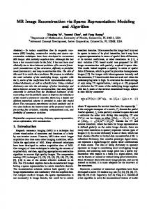
Figure 16: This amplification example was generated using a multi-resolution dictionary created from a real data-set. The original digital elevation map was taken from Australia at ε = 1 km resolution. The final sparse-terrain model has a resolution of ε = 4 m and was generated by applying 4 successive steps of amplification with a resolution increase factor of 4, yielding a total amplification factor of 256. Procedural texturing and vegetation were applied to outline ground details such as ridges and erosion patterns generated by the amplification process.
[CBC∗ 16] C ORDONNIER G., B RAUN J., C ANI M.-P., B ENES B., É RIC G ALIN , P EYTAVIE A., É RIC G UÉRIN: Large scale terrain generation from tectonic uplift and fluvial erosion. Computer Graphics Forum 35, 2 (2016). 2 [CMF98] C HIBA N., M URAOKA K., F UJITA K.: An erosion model based on velocity fields for the visual simulation of mountain scenery. The Journal of Visualization and Computer Animation – JVCA 9, 4 (1998), 185–194. 2 [CRT06] C ANDÈS E. J., ROMBERG J. K., TAO T.: Stable signal recovery from incomplete and inaccurate measurements. Communications on Pure and Applied Mathematics 59, 8 (2006), 1207–1223. 1
[MDH07] M EI X., D ECAUDIN P., H U B.: Fast hydraulic erosion simulation and visualization on GPU. In Pacific Graphics (2007), IEEE, pp. 47–56. 2 [MKM89] M USGRAVE F. K., KOLB C. E., M ACE R. S.: The synthesis and rendering of eroded fractal terrains. Computer Graphics 23, 3 (1989), 41–50. 2 [MZ93] M ALLAT S., Z HANG Z.: Matching pursuits with time-frequency dictionaries. Signal Processing, IEEE Transactions on 41, 12 (1993), 3397–3415. 5 [Nag98] NAGASHIMA K.: Computer generation of eroded valley and mountain terrains. The Visual Computer 13, 9-10 (1998), 456–464. 2
[DCV14] D IGNE J., C HAINE R., VALETTE S.: Self-similarity for accurate compression of point sampled surfaces. Computer Graphics Forum, Proc. Eurographics 2014 33, 2 (2014), 155–164. 3
[NLP∗ 13] NATALI M., L IDAL E. M., PARULEK J., V IOLA I., PATEL D.: Modeling terrains and subsurface geology. In Proc. Eurographics State Of The Art – EG STAR (2013), pp. 155–173. 2
[DGGK11] D ERZAPF E., G ANSTER B., G UTHE M., K LEIN R.: River networks for instant procedural planets. Computer Graphics Forum – CGF 30, 7 (2011), 2031–2040. 2
[Pey09] P EYRÉ G.: Sparse modeling of textures. Journal of Mathematical Imaging and Vision 34, 1 (2009), 17–31. 3
[EA06] E LAD M., A HARON M.: Image denoising via learned dictionaries and sparse representation. In In CVPR (2006), pp. 17–22. 3
[PGMG09] P EYTAVIE A., G ALIN É., M ÉRILLOU S., G ROSJEAN J.: Arches: A framework for modeling complex terrains. Computer Graphics Forum – CGF 28, 2 (2009), 457–467. 2
[EMP∗ 98] E BERT D. S., M USGRAVE F. K., P EACHEY D., P ERLIN K., W ORLEY S.: Texturing and Modeling: A Procedural Approach, 3rd ed. The Morgan Kaufmann Series in Computer Graphics. Elsevier, 1998. 2, 4 [GGG∗ 13] G ÉNEVAUX J.-D., G ALIN É., G UÉRIN É., P EYTAVIE A., B ENEŠ B.: Terrain generation using procedural models based on hydrology. Transaction on Graphics – TOG 32, 4 (2013), 143:1–143:13. 2, 10 [GGP∗ 15]
G ÉNEVAUX J.-D., G ALIN E., P EYTAVIE A., G UÉRIN E., B RIQUET C., G ROSBELLET F., B ENES B.: Terrain modelling from feature primitives. Computer Graphics Forum 34, 6 (2015), 198–210. 2, 3, 10
[GMM15] G AIN J. E., M ERRY B., M ARAIS P.: Parallel, realistic and controllable terrain synthesis. Computer Graphics Forum 34, 2 (2015), 105–116. 2 [GMS09] G AIN J., M ARAIS P., S TRASSER W.: Terrain sketching. In Proc. Symposium on Interactive 3D Graphics and Games – I3D (Boston, USA, 2009), ACM, pp. 31–38. 2 [HGA∗ 10] H NAIDI H., G UÉRIN É., A KKOUCHE S., P EYTAVIE A., G ALIN É.: Feature based terrain generation using diffusion equation. Computer Graphics Forum – CGF 29, 7 (2010), 2179–2186. 2 [JBPS11] JACOBSON A., BARAN I., P OPOVI C´ J., S ORKINE O.: Bounded biharmonic weights for real-time deformation. ACM Trans. Graph. 30, 4 (July 2011), 78:1–78:8. 3 [KMN88] K ELLEY A. D., M ALIN M. C., N IELSON G. M.: Terrain simulation using a model of stream erosion. Computer Graphics 22, 4 (1988), 263–268. 2 c 2016 The Author(s)
c 2016 The Eurographics Association and John Wiley & Sons Ltd. Computer Graphics Forum
[PH93] P RUSINKIEWICZ P., H AMMEL M.: A fractal model of mountains with rivers. In Proc. Graphics Interface – GI (Toronto, Canada, 1993), Canadian Information Processing Society, pp. 174–180. 2 ˇ ˇ [ŠBBK08] Š TAVA O., B ENEŠ B., B RISBIN M., K RIVÁNEK J.: Interactive terrain modeling using hydraulic erosion. In Proc. Symposium on Computer Animation – SCA (2008), pp. 201–210. 2
[TEC∗ 14] TASSE F. P., E MILIEN A., C ANI M.-P., H AHMANN S., B ERNHARDT A.: First person sketch-based terrain editing. In Proc. Graphics Interface – GI (2014), pp. 217–224. 2 [TGM12] TASSE F. P., G AIN J., M ARAIS P.: Enhanced texture-based terrain synthesis on graphics hardware. Computer Graphics Forum – CGF 31, 6 (2012), 1959–1972. 2 ˇ [VBHŠ11] VANEK J., B ENEŠ B., H EROUT A., Š TAVA O.: Large-scale physics-based terrain editing using adaptive tiles on the GPU. Computer Graphics and Applications – CG&A 31, 6 (2011), 35–44. 2
[XZZ∗ 14] X IONG S., Z HANG J., Z HENG J., C AI J., L IU L.: Robust surface reconstruction via dictionary learning. ACM Transactions on Graphics (Proc. SIGGRAPH Aisa) 33 (2014). 3 [ZDL∗ 14] Z HANG J., D ENG B., L IU Z., PATANÈ G., B OUAZIZ S., H ORMANN K., L IU L.: Local barycentric coordinates. ACM Trans. Graph. 33, 6 (Nov. 2014), 188:1–188:12. 3 [ZSTR07] Z HOU H., S UN J., T URK G., R EHG J. M.: Terrain synthesis from digital elevation models. Transactions on Visualization and Computer Graphics – TVCG 13, 4 (2007), 834–848. 2