Spatial and Temporal Spectra of Solar Convection

Solar MHD Theory and Observations: A High Spatial Resolution Perspective ASP Conference Series, Vol. **VOLUME**, 2006 Uitenbroek, Leibacher, and Stein

Spatial and Temporal Spectra of Solar Convection Dali Georgobiani,1 Robert F. Stein,2 and ˚ Ake Nordlund3 1 201-L

Arcadia Loop, Yorktown, VA 23692 of Physics and Astronomy, Michigan State University, East Lansing, MI 48824-2320, USA 3 Niels Bohr Institute for Astronomy, Physics and Geophysics, Juliane Maries Vej 30, DK–2100 Copenhagen, Denmark 2 Department

Abstract. Recent observations support the theory that solar-type oscillations are stochastically excited by turbulent convection in the outer layers of the solarlike stars. The acoustic power input rates depend on the details of the turbulent energy spectrum. We use numerical simulations to study the spectral properties of solar convection. We find that spatial turbulent energy spectra vary at different temporal frequencies, while temporal turbulent spectra show various features at different spatial wavenumbers, and their best fit at all frequencies is a generalized power law P ower = Amplitude × (f requency 2 + width2 )−n(k) , where n(k) depends on the spatial wavenumber. Therefore, it is impossible to separate the spatial and temporal components of the turbulent spectra.

1.

Introduction

It has been widely assumed that the turbulent energy spectrum, E(k, ν), where 1 2 v = 2

Z

dk dν E(k, ν),

can be separated into a spatial spectrum E(k) and a temporal spectrum χ k (ν) = χ, independent of wavenumber k: E(k, ν) = E(k) χ(ν). Solar turbulent convection is primarily driven at intermediate scales of granulation. At smaller scales k, between the basic energy input scale k0−1 and the dissipation scale kd−1 , there exists an inertial range where the spatial spectrum of the velocity field is scale independent and therefore has a power law form (Monin & Yaglom 1975). The theory of fully developed turbulence implies that the spatial turbulent energy spectrum E(k) should depend on k approximately as E(k) ∝ k −5/3 (Kolmogorov 1941). The temporal part of the turbulent spectrum, χk (ν), characterizes the time evolution of the correlation between velocities measured in two points separated by distance 2π/k. A Gaussian function, which assumes that two distant points in the turbulent medium are uncorrelated, is the usual choice for solar acoustic excitation calculations. 113

114

Georgobiani, Stein and Nordlund

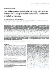
Figure 1. Left: the k − ν diagram of the gas pressure at one Mm below the surface. Note the broad convective power and narrow oscillation ridge. Right: Temporal power spectra of the vertical velocity at 0.25 Mm below the surface, for different k (in Mm−1 ). The spectra are a power law at small k and have a plateau at low frequencies for large k. Modes appear at small k near 3 mHz.

Our results show that the temporal components of the energy spectrum depend on the spatial wavenumber k, whereas the spatial components of the spectrum depend on the frequency ν. The best fit for the simulated temporal spectra is a generalized Lorentzian-like power law, where the width and the exponent are both functions of spatial wavenumber. These results indicate that the turbulent energy spectrum is not separable into spatial and temporal factors. 2.

Spatial and Temporal Spectra

We construct the energy spectra of vertical and horizontal velocity components, turbulent and gas pressure, and entropy. Fourier transforms of these variables in horizontal space and time (k − ν diagrams) are calculated at several depths: the τC = 1 surface, 100 km, 250 km, 500 km and 1 Mm beneath it. This corresponds to the depth range where p-mode excitation is most efficient (Stein & Nordlund 2001). The k −ν diagram contains acoustic mode ridges (Figure 1, left panel). We cut through these diagrams either at constant horizontal wavenumber or constant frequency to study the functional behavior of the variables with frequency and horizontal wavenumber. There are general trends characteristic of all these spectra. Temporal spectra for all variables and heights are typically a power law at large k and have a plateau at small k. Spatial spectra have an inertial range at low frequencies, which disappears with increasing frequency. The maximum of the spatial spectrum shifts to larger wavenumbers and decreases in amplitude with increasing frequency. The shape of the spectrum changes with depth. Figure 1 (right panel) shows the vertical velocity temporal spectra at 0.25 Mm, for several wavenumbers. The spectra at small k are power laws (acoustic modes are apparent near 3 mHz). As k increases, they develop a plateau at low frequencies. We compare these spectra with three commonly used analytic functions - Gaussian (GF), Lorentzian (LF) and Exponential (EF) (Samadi et al. 2005). We have made least square fits of these functions to the temporal spectra at several wavenum-

Spectra of Solar Convection

115

Figure 2. Temporal power spectra of the vertical velocity at 0.25 Mm beneath the surface. Left: at k = 4 Mm−1 , compared with analytic fits GF, LF and EF. Right: at k = 4 and 10 Mm−1 , with a generalized power law fit.

bers k. In addition, power-law fits were made for the frequency range where the spectra approach power-law behavior. Figure 2 (left panel) shows the temporal power spectrum of the vertical velocity at k = 4 Mm−1 . The GF, LF and EF fit well at low frequencies, but deviate significantly at high frequencies; on the contrary, a power law cannot fit the low frequency region, but represents the high frequency range quite well. The transition to a power law happens at higher frequencies for higher wavenumbers (Figure 1). The best fit for the temporal power spectrum at all frequencies is a generalized power law function: P ower = A × (ν 2 + w2 )−n , where A is amplitude, ν is the frequency, w is width and n is an exponent (n = 1 corresponds to a Lorentzian) (Figure 2, right panel). We made such fits for all five variables at various spatial wavenumbers and depths and determined the dependence of the parameters on wavenumber (e.g. Figure 3). For all five variables, the width of the plateau at low ν tends to increase with increasing k. Their power-law exponent tends to approach a Lorentzian (n=1) at large depth and be steeper near the surface. The spatial spectra of all variables, at depths of 0.5 Mm and below and at low frequencies, increase with increasing horizontal wavenumber k at small k, reach a maximum and then decrease in a Kolmogorov -5/3 power law inertial range, ending in a more rapidly decreasing damping tail. With increasing frequency, the wavenumber of the maximum in the spectrum shifts to larger k, eventually reaching the damping range and wiping out an inertial range (e.g. Figure 4, left panel). For the vertical velocity, the energy (in the p-mode frequency range) is a maximum between 9 and 12 Mm−1 , which corresponds to a horizontal scale of about 0.6 Mm. From Figure 4 (right panel), it is apparent that the frequency-averaged spatial power spectra, e.g. Samadi et al. (2003a), do not possess a Kolmogorov inertial range, unlike the single-frequency spatial spectra at low frequencies (Figure 4, left panel).

116

Georgobiani, Stein and Nordlund

Figure 3. Exponent (power) and width of the generalized power law best fit the temporal spectrum of the vertical velocity, at different depths, as a function of the horizontal wavenumber.

Figure 4. Left: vertical velocity spatial spectra at various ν (in mHz), at 0.5 Mm below the surface. The inertial range extends from k ' 3 Mm−1 to k ' 15 Mm−1 , and vanishes with increasing ν. High k decaying tail is due to the numerical damping. At low k, spectra behave as k 2 . Right: frequency averaged spatial spectra of the vertical velocity at different depths. Thin solid line represents the power law of -5/3 characteristic for the turbulent cascade. There is no clear inertial range at this resolution.

Spectra of Solar Convection 3.

117

Conclusion

We have calculated the spectra of several variables from realistic simulations of solar convection. Our most important conclusion is that temporal spectra are different at different spatial wavenumbers k. This means that it is impossible to separate the spectral power into a spatial factor E(k) and a temporal factor χ(ν). One should be cautious when using functional forms of these spectra in the calculations of stellar oscillation amplitudes or excitation rates. For example, the widely used Gaussian function does not represent any of the variables well, except at very low frequencies (see also Samadi et al. 2003b). We have found a function which, with the proper choice of its exponent and width, provides a good fit for the whole frequency range. Exponents and widths vary for different variables, at various heights and for different wavenumbers. These facts should be taken into account when using a functional representation of the temporal spectra. Time-averaged spatial spectra, e.g. Chan & Sofia (1996), do not show an extended inertial range. The spatial spectra at individual frequencies have different behavior, depending on a frequency. At high frequencies, their maxima are shifted to higher wavenumbers, and the decaying tails at high k are caused by viscous damping. At low wavenumbers, spatial spectra behave as power laws and agree with observations. Our results suggest that the mode excitation occurs not on the scale of granulation (one Mm), but at smaller scales, about 0.5 – 0.75 Mm where the convective power is largest. These results are consistent with the idea of wave excitation occurring in the narrow turbulent downflows, which is supported by observations (Goode et al. 1998). The rates of the energy input into the solar-like oscillations are very sensitive to the models of the turbulent energy spectra (Samadi et al. 2001). For the Sun, it should be possible to deduce the analytical forms of the spatial and temporal spectra from the observations of the solar granulation (although, cf. Nordlund et al. (1997)). It is not possible to obtain similar information for other stars. Therefore, it would be useful to analyze the spectra from the stellar simulations in the same manner as for the solar simulations (Samadi et al. 2005). Asteroseismic observations will supply more information on the excitation and damping rates; this will help to better understand the stellar turbulent convection. Acknowledgments. DG would like to express her gratitude to RFS and the workshop organizers. This work was supported by grants AST0205500 from NSF and NAG512450 and NNG04GB92G from NASA. Their support is greatly appreciated. The calculations were performed at the National Center for Supercomputing Applications (which is supported by NSF) and at Michigan State University. ˚ AN acknowledges support from the Danish Natural Science Research Council (SNF) and from the Danish Center for Scientific Computing (DCSC). References Chan, K. L. & Sofia, S. 1996, ApJ, 466, 372 Goode, P. R., Strous, L. H., Rimmele, T. R., & Stebbins, R. T. 1998, ApJ, 495, L27 Kolmogorov, A. N. 1941, Doklady Akad. Nauk SSSR, 32, 16 Monin, J. S. & Yaglom, A. M. 1975, Statistical Fluid Mechanics: Mechanics of Turbulence Vol. 2, (Cambridge: MIT Press)

118

Georgobiani, Stein and Nordlund

Nordlund, A., Spruit, H. C., Ludwig, H.-G., & Trampedach, R. 1997, A&A, 328, 229 Samadi, R., Georgobiani, D., Trampedach, R., Goupil, M. J., Stein, R. F., Nordlund, ˚ A., & Fernandes, J. 2005, A&A Samadi, R., Goupil, M.-J., Lebreton, Y., & Baglin, A. 2001, in ESA SP-464, SOHO 10/GONG 2000 Workshop: Helio- and Asteroseismology at the Dawn of the Millennium, ed. A. Wilson (Noordwijk: ESA) 451 Samadi, R., Nordlund, ˚ A., Stein, R. F., Goupil, M. J., & Roxburgh, I. 2003a, A&A, 403, 303 Samadi, R., Nordlund, ˚ A., Stein, R. F., Goupil, M. J., & Roxburgh, I. 2003b, A&A, 404, 1129 Stein, R. F. & Nordlund, ˚ A. 2001, ApJ, 546, 585