Spatial and temporal variability in streamflow ... - Science Direct

Journal o f Hydrology, 142 (1993) 137-166 Elsevier Science Publishers B.V., Amsterdam

137

t21

Spatial and temporal variability in streamflow generation on the West Fork of Walker Branch Watershed D a v i d P. G e n e r e u x '~, H a r o l d F. H e m o n d a a n d P a t r i c k J. M u l h o l l a n d b

aDepartment of Civil Engineering, Building 48, Room 4191 Massachusetts Institute of Technology, Cambridge, MA 02139, USA bEnvironmental Sciences Division, Oak Ridge National Laboratory, P.O. Box 2008, Oak Ridge, TN 37831-6036, USA (Received 20 February 1992; revision accepted 16 June 1992)

ABSTRACT Genereux, D.P., Hemond, H.F. and Mulholland, P.J., 1993. Spatial and temporal variability in streamflow generation on the West Fork of Walker Branch Watershed. J. Hydrol., 142: 137-166. Spatially intensive measurements of streamflow were used to document the spatial and temporal variability in streamflow generation on the West Fork of Walker Branch Watershed, a 38.4 ha forested catchment in Oak Ridge, Tennessee. The study focused on a 300 m section of a small stream, and covered a wide range of flow conditions (Qw~ir, streamflow at the basin outlet, varied from about 350 to 3500 1 rain t ). There was enormous spatial variability in the stream inflow, down to the finest scale investigated (reaches 20 m in length). Lateral inflow to longer reaches (60-130 m) was linearly correlated with Qw~lrover the full range of flows studied, making it possible to estimate the spatial pattern of stream inflow from measurement of Q~.~ alone. The heterogeneous nature of the karstic dolomite bedrock was the dominant control on the observed spatial variability in streamflow generation. This thesis is consistent with the results of field investigations using natural tracers, reported in a companion paper. Bedrock structure and lithology may affect streamflow generation directly (via water movement through fractured rock), and indirectly (by influencing the slope and thickness of the overlying soil). While the West Fork contains all the topographic and surface hydrologic features of larger basins (ridge tops, valleys, hollows, spurs, ephemeral and perennial stream channels), it covers an area which is relatively small with respect to the bedrock heterogeneity. Therefore, while the hydrologic processes observed on the West Fork are no doubt typical of those occurring elsewhere in karst terrain, the particular patterns of spatial and temporal variability observed are somewhat specific to the study site.

INTRODUCTION

The study of streamflow generation is an important topic in environmental science, both because of its direct relevance to the hydrologic cycle and Correspondence to: D.P. Genereux, Department of Geology and Drinking Water Research Center, Florida International University, PC-327A, University Park, Miami, F L 33199, USA.

0022-1694/93/$06.00

© 1993 - - Elsevier Science Publishers B,V. All rights reserved

138

D.P. GENEREUX ET AL.

because the water quality of streams is directly affected by the nature of the flowpaths supplying water to the streams. Consideration of spatial variability is a necessary component of streamflow generation studies, both in the field and on the computer. Since the number of sites at which measurements can be made is always limited in practice, it" is useful to identify areas of high streamflow production so that measurements may be concentrated in those areas. In addition, it is essential to have some idea how representative a measurement is if it is used to infer the behavior of the surrounding area. Also, comparison of the spatial pattern of stream inflow with that of other watershed parameters can elucidate the controls on streamflow generation. For a study site in southern England, Anderson and Butt (1978) found that all stream reaches of high lateral inflow were adjacent to hillslopes with concave, hollow-shaped topography. Concave topography led to convergent drainage pathways, which in turn led to saturated conditions and higher overall streamflow production in the hollows. Spatial variability in streamflow generation is also a concern in modelling. Wood et al. (1988) proposed the notion of a "Representative Elementary Area" (REA), the smallest basin size for which the variance of a basin output or response (e.g. volume of storm runoff for a particular rain event) is a minimum. The REA would be 'a fundamental building block for catchment modelling' (Wood et al., 1988, p. 31) since at this scale the particular pattern of heterogeneity in the study basin becomes unimportant, and the basin response can be analyzed in terms of the statistics of the underlying parameter distributions. Thus, an estimate of the REA would be useful in deciding the appropriate basin size for a modelling study. This paper describes measurements of the spatial variability in streamflow generation on the West Fork of Walker Branch Watershed, a forested watershed in Oak Ridge, Tennessee. Chemical dilution stream gauging was used to determine streamflow at a number of points in the small stream draining the study site, over a wide range of flow conditions. A companion paper (Genereux et al., 1993) reports the results of simultaneous work with natural tracers. STUDY SITE The West Fork of Walker Branch has an area of 38.4 ha and an elevation ran~'e of 78 m (Fig. l). Precipitation is measured with two weighing-type rain gauges on the ridge top; average annual precipitation is 140 cm. Streamflow at the basin outlet is monitored by means of a 120° V-notch weir with automatic stream stage recording (5 min interval). Vegetation is dominated by oak and hickory, with scattered pines on the ridges and mesophytic

SPATIAL AND TEMPORAL VARIABILITYIN STREAMFLOWGENERATION

139

WALKER BRANCH W A T E R S H E D - WEST FORK

A

A

9 --

O0 .]

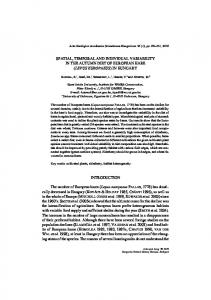
Fig. I. Contour map of the study site. Major stream sampling sites are indicated by triangles; stream sites are designated with the prefix 'WB' followed by their distance upstream of the weir in meters (e.g. WB300 is the point 300 m upstream of the weir). The two unlabeled triangles represent WBI00 and WB242. Solid lines normal to the elevation contours and passing through WB60, WBI70, and WB300 indicate the boundaries of'apparent contributing areas' (ACAs) for the stream reaches they define (that is, contributing areas defined in the usual way, on the basis of topography).

hardwoods, such as tulip poplar and beech, near the stream channels (Johnson, 1989). The West Fork is located on the southeast slope of Chestnut Ridge, one of many NE-SW-trending subparaUel ridges in this area of the southern Appalachians. Bedrock consists of highly fractured dolomite (with some chert beds) of the Knox Group. Strata dip to the southeast at about 35 ° and strike along the long axis of Chestnut Ridge (roughly N 55° E), approximately normal to the study stream on the West Fork (Crider, 198 i; Lee et al., 1984). The West Fork is underlain by three different formations of the Knox; from oldest to youngest (i.e. going southeast along the perennial stream towards the weir) they are the Chepultepec, the Longview and the Kingsport dolomites (Fig. 2). The Longview is much thinner than the other two formations and is more resistant to weathering because of its significantly higher chert content (Lietzke et al., 1989; Lietzke, 1990). All three formations are highly fractured;

140

D.P. GENEREUX ET AL.

0 0

~ ~

600 f t

i

•

250 m 10 f-'oat Contours

Welre

Pored roocl/trall Per,':nnlal/ephameral stream

........ W a t e r s h e d

boundary

Fig. 2. Map of Walker Branch Watershed showing the different bedrock formations. The West Fork catchment shown in Fig. I is the triangular basin occupying the left side of this map (the East Fork, on the right, makes up the rest or Walker Br,'mch).

a study involving measurement of 210 fractures in outcrops on Walker Branch (the West Fork ant, the adjacent 59.1 ha East Fork) found that fractures cluster in two common orientations, roughly perpendicular to, and parallel to, the local bedrock strike (Crider, 1981). In addition to being more numerous, fractures with these orientations were also found to be the only fractures 'solutionally enlarged to conduits in outcrops on the West Fork' (Crider, 1981, p.85). As discussed below and again later in the paper, these fractures are hydrologically significant in allowing groundwater movement across surface topographic divides. Soils on the West Fork are mainly Ultisols (mostly of the Paleudult suborder), with one small band (< 5% of the watershed area) of Alfisols (suborder Hapludalt) along the east side of the lower 150 m of the perennial stream (Lietzke, 1990). Both Ultisols and Alfisols show the effects of clay translocation: an eluvial E horizon from which clay has been removed overlies an argillic Bt horizon where the clay particles have been deposited (Soil Conservation Service, 1975). The dominant clay mineral on the West Fork is kaolinite (10-40% of the clay fraction), with vermiculite and mica present in smaller amounts. The primary distinctions between Ultisols and Alfisols are

SPATIAL AND TEMPORAL VARIABILITY IN STREAMFLOW GENERATION

14l

chemical and mineralogical, rather than structural or physical. According to Fanning and Fanning (1989, p. 264), 'Most Alfisols differ from Ultisols in having a naturally higher base saturation (> 35% for the former, < 35% for the latter) - - thus, commonly higher pH values - - generally lower chromas and yellower hues for the well-drained counterparts, and clay usually containing less l:l and more 2:1 layer silicate minerals'. Narrow zones of Entisols, soils which lack distinct pedogenic horizons, are found along the stream channels (both ephemeral and perennial). In many places c n the West Fork a thick layer of saprolite (residual clayey material formed in place by weathering of the dolomite bedrock) lies between the 1-2 m thick forest soil and the bedrock. This saprolite consists mainly of kaolinite (30-55%), mica (10-25%), vermiculite (5-20%) and iron oxide (2-8%) in the clay size ( < 2 # m ) fraction (Lee et al., 1984). Chert fragments are common, in places where a chert bed in the original bedrock has partially weathered but the surrounding dolomite has completely weathered to saprolite. In places on the western and northern ridge tops around the West Fork, the saprolite is nearly 30 m thick. Over much of the eastern side of the perennial stream valley (the same general area covered by Alfisols), there appears to be little or no saprolite (small rock outcrops can be seen running upslope from the stream channel; well points have been driven to refusal within 2 m of the ground surface). The saprolite thickness is unknown or poorly known for much of the watershed. Previous studies have shown that a perched saturated zone often develops above the soil/saprolite interface during storms (e.g. Wilson et al., 1990). While the saprolite may be much thicker than the overlying soil in some places, it has a much lower maximum possible transmissivity than the soil Cmaximum possible transmissivity~ refers to the transmissivity of the layer saturated over its entire thickness). The hydraulic conductivity of saprolite was measured in three different depth intervals (2°5-3, 6-12 and 21-30 m) at a site about 6 km west of the West Fork on Chestnut Ridge (Ketelle and Huff, 1984). Geometric mean conductivities were 6.1 x l0 -8 m s -I at 2.5-3 m (21 field measurements), 2.0 x 10 -8 m s-t at 6-12 m (19 field measurements), and 6.3 x l0 -I° m s - ' at 21-30 m (eight laboratory measurements). Assigning these three conductivity values to three somewhat arbitrarily chosen layers (1.5-4.5, 4.5-16 and 16-30 m below ground surface) gives an estimate of 4.2 x l0 -7 m 2 s-~ for the maximum possible transmissivity ofthe saprolite. Even if the laboratory measurements of hydraulic conductivity for the deepest layer underestimate the field scale value by a factor of l0 (which is possible), the effect on overall transmissivity is minor (it increases to 5 x 10- 7 m 2 s- ~). An overlying soil consisting of a 1 m thick B horizon (hydraulic conductivity of 10 -5 to 10 -4 m s -t (Luxmoore et al., 1981)) and a 0.5 m thick A horizon

142

D.P. G E N E R E U X ET AL.

(hydraulic conductivity of about 10 -4 m s-t (Peters et al., 1970)) would have a maximum possible transmissivity of 6 x 10 -5 to 1.5 x 10 -4 m 2 s -~, 140-360 times larger than that of the 28.5 m thick saprolite. Streamflow and rainfall data for the West Fork indicate that the watershed receives subsurface inflow from outside its topographic boundary. For the 12 years from 1969 through 1980, the average difference between annual rainfall and annual runoff at the weir was 34cm (SD = 16cm, n = 12). The best estimates of annual evapotranspiration (based on the average difference between rainfall and runoff for a number of watersheds in the Oak Ridge area) are about 73 cm (McMaster, 1967; Tennessee Valley Authority (TVA), 1972). Thus, the West Fork stream seems to be receiving about 1.5 x 105 m 3 of water each year (39 cm x 38.4 ha) from outside the West Fork boundary. Solutionally enlarged fractures and cavities in bedrock are the most likely conduits for this interbasin transfer. METHODS

Chemical dilution gauging was used to determine the streamflow rate at a number of sites in the perennial stream channel; experiments spanned the range of Qwo~r(streamflow at the weir) from 354 to 3457 1min -t . The five main sites for streamflow determination are indicated with triangles in Fig. I. The sites, each named with the prefix 'WB' followed by its distance upstream of the weir in meters, are WB300, WB242, WBI70, WBI00 and WB60. A flume installed in the stream channel at WB300 allowed us to check (or, occasionally, forego) chemical dilution streamflow measurements at that site. in addition to these five main sites, measurements were occasionally made at six additional sites (WB280, WB260, WB220, WBI40, WBI20 and WB80) in order to get more detailed information on the spatial structure of the stream inflow. The chemical dilution methodology involves a one-dimensional steadystate analysis (e.g. Genereux and Hemond, 1990). A 50 1 Mariotte bottle was used to inject a concentrated (2.7-3 mol l-~ ) NaCl solution into the stream at a steady rate. The injection site varied, but was always 12-17 m upstream of the nearest measurement site. Since the channel was laterally well mixed (no vertical or horizontal tracer gradients), the streamflow Q at a stream measurement site was given by the simple steady-state relationship: Q = QoCo/C

where Q0 and Co are the injection rate and concentration of the NaCl tracer solution, respectively, and C is the steady-state tracer C1- content of the streamwater at the site.

SPATIAL AND TEMPORAL VARIABILITY IN STREAMFLOW GENERATION

143

C values were estimated by two different means: field measurement of the specific conductance (7) of the streamwater and laboratory measurement of the CI- content (S) of the streamwater. Before beginning the NaC1 injections the background specific conductance of the streamwater (Tb) was determined at each measurement site. A battery powered hand-held conductivity meter (Cole-Parmer Instrument Co. model 1481-60) with a gold dip cell was used; the meter automatically corrected the measured conductance to an equivalent value at 25°C. Measurements were generally taken 30 s apart for several minutes in order to determine if there was any drift in ~b. Prior to the three highest flow experiments ~b was slowly drifting upward at WB170, WBI00 and WB60. The ~'b drift rate at the three sites was noted and used to extrapolate ~'b forward in time to when 7~ (the steady-state plateau 7 value) was measured, in order to better estimate the background specific conductance under the plateau. The dril~ in 7b was associated with a slow decrease in Qw~r (maximum rate of C~r decrease was - 1 . 7 % h -I, during the highest flow experiment on 18 t,~.arch 1990). Strictly speaking, the chemical dilution methodology employed here requires that the streamflow be steady. In practice, the small drop in streamflow observed during the highest flow experiments introduces a negligible uncertainty into the calculated Q values (see Appendix). After measuring )'b at a particular site, water samples (two or three) were collected for analysis of background C1- content (Sb); the unfiltered samples were collected by rinsing and filling small polyethylene bottles with streamwater. We did not attempt to measure drift in Sh because both Sb (about 0.02 mmol l -~) and changes in Sb associated with changes in streamflow ( l0 min (or ~ on the plateau was drifting at the same rate as 7b). After the specific conductance reached steady state three or four water samples were collected for CI- analysis (S~). Both S, - S b and ~,~-~'b were used as measures of C in calculating Q values with eqn. (1). Q0 values for use in eqn. (l) were measured in the field with a stopwatch and graduated cylinder; Co for each tracer solution was determined from the known amounts of NaC! and distilled water used to prepare the solution. In determining the uncertainty in Q, the uncertainties in Q0 and Co were negligible compared with the uncertainty in C (see Appendix).

144

D.P. GENEREUX ET AL.

4

•

.'.,

"

m~k

Fig. 3. Specific conductance data for the experiment of 4 October 1989. The steady NaCI injection was begun at time zero.

Chloride concentrations (both S~ and Sb) were measured with an automated ferricyanide method (U.S. Environmental Protection Agency (EPA), 1983), using a Technicon T R A A C S 800 auto-analyzer. The steadystate (S~) samples were diluted with doubly distilled water prior to analysis, to bring their CI- contents into the range spanned by the calibration standards. The difference S~ - Sb was calculated and used directly as C in eqn. (1). In using 7~--~b values in eqn. (1) to determine Q values, it is necessary to convert the 7~ -~b value from at least one measurement site to an equivalent CI- concentration. Measuring the specific conductance of the tracer solution (~0) and expressing the tracer injection rate as Q070 (instead of QoCo)would not suffice because the relationship between 7 and NaCI concentration is not linear o~,er the full range from 70 (roughly i.7 x 105 llS cm -~ ) to ~,~-~,~ (typically 100-400 ItS cm- t ); therefore Q0)'0 =/=Q(~ - 7b). Data from Jones (1912) was used to convert the 7 ~ - 7b value from the first measurement site (that farthest upstream; either WB300 or WB242) to a CI- concentration. A linear regression of Jones' five data points (at 25°C) in the range 29 < I' < 880 ItS cm-~ gave the following relationship: C = 8.91 x 10-6~,-2.97 x 10 -s

(r = 0.99997)

(2)

where C is concentration in mol 1-1 and 7 is specific conductance in pS cm-I. After using eqn. (2) to convert the 7~-7b value from the first site to a CIconcentration, and using eqn. (1) to calculate Q at that site, streamflow values at the other sites downstream were calculated by using ~'s -~'b values directly in eqn. (1): Q/

=

O l ()'s - - )'b )l /()'s - - Tb )i

(3)

145

SPATIAL AND TEMPORAL VARIABILITY IN STREAMFLOW GENERATION

TABLE 1 Lateral inflow to six reaches of the study stream during 13 chemical dilution experiments Qweir

Date

Lateral inflow (1 min- ~)

(I m i n - i )

302 354 395 a 411 680 709 a 722 1050 1148~ 1368 1447 2749 3457

8/9/89 1/11]89 20/7[90 28]8/90 13/4/90 12]4/90 8•4/90 7]3/90 6/3/90 4/10]89 7/5]90 17111/89 18/3/90

1

2

3

4

37 53 60 161 162 178 350 380 526 537 1055 1640

39 33 30 37 70 55 46 97 110 105h 122 125 h

203 248 204 249 276 251 304 278 254 323 323 466 h

13 54 23 29 56 65 71 87 79 15 54 97 h 61 h

5

6

14 13 7 11 2 20 5 0

21 26 78 166 138 150 260 326 (468)

55 82 b 151

403 1081 1007

a The experiments represented in Fig. 4, during which measurements were made at additional sites. h Lateral inflow values which are based on S data lone (7 data are not considered reliable here; see text). Stream reaches I-6 are as follows: 1, above WB300; 2, WB300-WB242; 3, WB242-WB! 70; 4, WBI70-WBI00; 5, WBI00-WB60; 6, WB60-WB0. No measurements were made at WB60 on 4 October 1989; a total lateral inflow value for WBI00-WB0 is given in parentheses for that day.

where the subscripts 1 and j refer to the measurement site farthest upstream and a site downstream of it, respectively. This is possible because the conductance-concentration relationship for aqueous NaCl solutions is highly linear over the relatively small range of "/s--Yb values (100-400#S cm -t) spanned by the stream sites (see eqn. (2)). Lateral inflow to a given stream reach was determined as the difference in streamflow rates at the upstream and downstream ends of the reach. There are two estimates of Q for each measurement site during each experiment (one based on ? data, the other on S data), and hence two estimates of the lateral inflow to each reach during each experiment (except for the 6 March 1990 experiment, when S data were not collected). In general, the lateral inflow determinations based on ? data were in good agreement with those based on S data, and the two were simply averaged. The few exceptions (marked by asterisks in Table 1) were cases in which the Ydata appeared to give unrealistic

146

D.P. GENEREUX ET AL.

results at high flow. For example, ), data gave lateral inflow rates of about 400 I min-i for WBI70-WB100 and WBI00-WB60 when Qw~ir was 2749 1 min-~, much higher than the lateral inflow to these reaches at Qw~ = 3457 1 min-1. Specific conductance data also suggested a lateral inflow rate of about 13 l min-I for WB300-WB242 at Qwe~r = 3457, a value roughly ten times lower than that indicated by the S data for the same experiment, and by both the y and S data when Qweir was 2749 1 min -~ . These few seemingly anomalous results could be due in part to the random noise associated with calculating a small difference between two much larger numbers. However, the fact that all the anomalous numbers are based on 7 data at high flow, which is known to be potentially problematic because of drift in 7h, suggests there is an important non-random aspect to the observed behavior. Perhaps the }'b measu~ements prior to the start of the injections did not accurately characterize the 7b drift occurring later in the experiments, near steady state. Because of these anomalies, lateral inflow values were based on S data alone for six cases. RESULTS

Voriabi6ty There was considerable spatial variability in streamflow generation on the West Fork at all spatial scales investigated (reaches from 20 to more than 100m in length). Figure 4 shows lateral inflow to the perennial channel between WB300 and the weir on three different days with different Q,,~r values. The reach between WB220 and WB! 70 stands out as an important contributor, especially at low flow. Most of the inflow in this reach is due to two springs ($3 and S3A) at the base of a large hollow on the east slope. Perhaps the most dramatic feature of these data is the dynamic behavior of lateral inflow between WB60 and the weir. While relatively unimportant at low flow, lateral inflow to this 60 m reach increases rapidly with total streamflow, and eventually becomes the largest contributor to inflow in the perennial stream channel. Data from Huff et al. (1982) also show the importance of this reach, though this was not discussed in their paper. Their study involved the release of 9.75 mCi of 3H (as tritiated water) to the stream. Streamflow was determined at several sites from WBI81 to WB66; Q,,~r was 371 1min -~ . Figure 5 is similar to a graph in figure l of Huff et al. (1982), but is redrawn to include the lateral inflow between WB66 and the weir (using the Qwe~rvalue given in their paper). There is more lateral inflow in this 66 m reach (98 1 min -~ ) than in their I I 5 m study reach, WBI81-WB66 (82 l min-I). Data covering a wider range of flow at a somewhat coarser spatial

SPATIAL AND TEMPORAL VARIABILITY IN STREAMFLOW GENERATION Stream

inflow

147

on the West Fork

Owe,f= t 1 4 8 l i t e r s / m i n

5~ 4

3 2

1 ~D qJ

0

I

0

200

300

6

E ~3_

loo

Q.eif = 709 l i t e r s / r a i n 5

E

4

3 v

2 o E

I

CO O

0

Og

,

0

1QO

I

2O0

300

6

Q.~,r = 395 l i t e r s / r a i n 5 4

3 2 I

0 0

100

200

,l

300

Meters upstreom of wew

Fig. 4. Lateral inflow to the study stream between WB300 and the weir on three different days with different

O~,eir values.

resolution (40-70 m reaches) are given in Table 1. Reach lateral inflow correlated well with Qwe~,. Treating the channel section between WB300 and WB60 as two reaches instead of four removes some of the random scatter associated with calculating a small lateral inflow as the difference between two large streamflow numbers. Figure 6 shows linear regressions of lateral inflow vs. Qweir for four stream reaches comprising the entire West Fork surface

148

-

D.P.

"

¢

/

GENEREUX

ET AL.

]

t

"~,

• =

371

I

liters/rain

I

'C

J

!

.c

~

;

~

~

!i:

'

¢~

From Hu'~fet

i

1,nO

j 300

20C

iVete,-s ,~pstr~orr, of ~,ei,

Fig. 5. Lateral inflow data of Huffet al. (1982) between WBI81 and the weir.

drainage system: above WB300, WB300-WB 170, WB 170-WB60 and WB60WB0 (WB0 is the weir). Table 2 gives the parameters for these four regressions. An important limitation to keep in mind is that the lateral inflow data were collected during times of steady flow, or slowly decreasing flow on the falling limbs of hydrographs. The relationships in Table 2 and Fig. 6 would not necessarily hold as well during the rising limbs of hydrographs. The relationships between lateral inflow and Qweir were highly linear over a wide range of flow. The regression parameters (slope and intercept) are of interest because they contain the basic information about where streamflow is generated on the watershed. The intercepts of the lines in Fig. 6 show that at low flow typical of the late summer ( ~, 350 1 min-' ), most of the streamflow leaving the West Fork is generated between WB300 and WBI70 (much of that in springs $3 and S3A). The slopes of the lines show that as Qw~r increases, 49% of any increase is generated upstream of WB300 (mainly in the .

.

.

.

.

.

.

.

.

.

.

.

.

.

,

,

,

[

]

/

t ,b ,'. ',','I':'(~

":

A *I°' ',

~' i'

I

~I ',~

"1

i

L I

:,qd: ; "' t

i

~.-~

!~,, !~ . . . . . .

t . . . . lr~ !

,,%,

¢,,,,r

' .... ',lit,,r

,~,,r

,

Fig. 6. Linear regressions of lateral inflow vs. Q.~,~ for four stream reaches on the West Fork. Regression parameters are given in Table 2.

SPATIALAND TEMPORALVARIABILITYIN STREAMFLOWGENERATION

149

TABLE 2 Parameters for linear regressions of lateral inflow vs. Q~,eir for four reaches; n is the n u m b e r o f points used in the regression Reach

Above WB300 WB300-WB 170 WB i 700-WB60 WB60-WB0

Regression parameters Slope

Intercept

r, ~orr. coeff,

n

0.4912 0.0973 0.0529 0.3575

- 162.9 236.5 31.5 - 89.9

0.9937 0.9442 0.9724 0.9786

12 12 1! 11

ephemeral channel system), 10% is generated between WB300 and WB170, 5% between WBI70 and WB60 and 36% between WB60 and the weir. A dramatic demonstration of spatial variability is provided by using the regressions in Fig. 6 and the streamflow data from the weir to estimate the "apparent runoff' from the 'apparent contributing areas' (ACAs; see caption of Fig. l) delineated in Fig. I. For the period l September 1989-31 August 1990 the total amount of streamflow passing the weir was 132cm (total volume of streamflow divided by 38.4 ha), or 965 l min-I averaged over the 12 month period; precipitation was 168 cm. (These data suggest an interbasin transfer into the West Fork, equal to total streamflow plus average evapotranspiration (73 cm; see 'Study site' section of paper) minus precipitation, of about 37 cm for the 12 month period.) Using this average Qweir of 965 1minin the regression lines of Fig. 6 gives an estimate of the average lateral inflow rate to each stream reach for the 12 month study period. Dividing the average volumetric lateral inflow rate for each reach by the size of its ACA yields an estimate of the depth of'apparent runoff' from each ACA. Since flows under the rising limbs of hydrographs account for a small proportion of the year's total flow, results should not be greatly affected by possible hysteresis in the spatial distribution of stream inflows (i.e. by the possibility that the spatial distribution of stream inflows during rising flow is not accurately represented by data in Fig. 6). Results show tremendous variability (Fig. 7), with the bulk of the watershed (upstream of WB300) apparently generating only 55cm of streamflow and the small area just above the weir seemingly producing an amount of streamflow equivalent to about 6.5 times the total depth of precipitation. These apparent runoff values, and the regression equations from which they were calculated, clearly reflect the movement of subsurface water across surface topographic divides. Some of the streamflow generated dowr stream of WB300 may be due to groundwater movement across the downstream

150

D.P. GENEREUX ET AL.

L-

.',-'

.'.--

Fig. 7. "Apparent runoff' from four "apparent contributing areas" (ACAs) comprising the West Fork, I September 1989-31 August 1990. Precipitation during this 12 month period totaled 168cm. The sizes of the four ACAs are as Ibllows: above WB300, 29.5 ha; WB300-WBI70, 4.47 ha" WBI70-WB60, 3.15 ha: WB60-WBO, 1.24 ha. The horizontal dashed line represents the average for the entire 38.4 ha West Fork.

boundary of the ACA above WB300, within the West Fork. However, the overall water balance for the West Fork indicates that much of the stream inflow must be due to groundwater movement into the West Fork from outside. Controls

Streamflow data at different spatial scales indicate the importance of groundwater movement across surface topographic divides, including a net transfer into the West Fork from outside. It is much more likely that such transfers take place within the bedrock than in the overlying regolith (soil plus saprolite). Significant water movement through the saprolite is unlikely given its low transmissivity. The overlying 1-2 m thick soil mantle has a much higher transmissivity, but it follows the topography and hence is not a logical candidate for a medium in which there are significant water fluxes across topographic divides. On the other hand, the permeable karst nature of the bedrock is well established, by observations both in outcrop within the West Fork (Crider, 1981) and in boreholes outside the West Fork but within Chestnut Ridge (e.g. Ketelle and Huff, 1984). Of 20 boreholes drilled into bedrock on west Chestnut Ridge (about 6 km west of the West Fork, in the same Knox Group rocks), most penetrated some weathered, cavitose bedrock, and seven penetrated more than 30 m ofcavitose bedrock (vertical dimensions ofcavities were 0.3-5 m) without encountering sound, unweathered rock (Ketelle and Huff, 1984). Crider's (1981) observations of bedrock fractures and cavities within the West Fork have already been mentioned. Thus, direct physical

SPATIAL AND TEMPORAL VARIABILITY IN STREAMFLOW GENERATION

151

observations of geologic media at the study site suggest that the bedrock carries the bulk of the interbasin transfer, a substantial volume of water corresponding to ~ 3 7 c m of runoff during the 12 month study period. It is, of course, possible that some of the groundwater moving through the bedrock as fracture flow fell as precipitation on the West Fork (all the bedrock groundwater flow need not be interbasin transfer, though it is likely that nearly all the interbasin transfer is bedrock groundwater flow). Tracer data are used to pursue this point in a companion paper (Genereux et al., 1993). Groundwater movement to the study stream in bedrock fractures should affect the spatial variability as well as the magnitude of stream inflows. Relative to a case with no bedrock groundwater inputs, the spatial variability of stream inflows would be increased by water inputs from irregularly spaced fractures. Springs $3 and S3A are examples of this effect. $3 and S3A are large perennial springs with relatively constant flow (about 100 1 min -~ and 50 1 min -I , respectively), constant chemistry (the water is saturated with respect to dolomite) and constant temperature (approximately equal to the mean annual air temperature, 14.5°C). These characteristics indicate that $3 and S3A are almost certainly sites where bedrock groundwater discharges into the study stream. Additional evidence for the bedrock origin of outflow from $3 and S3A comes from the lack of a soil saturated zone near the springs. Five well points were driven into the soil (four to refusal) between $3 and S3A, alotig a line roughly parallel to, and about 3 m from, the streambank. No water table was ever found in the downstream three; the two farthest upstream were installed side by side near S3A (one 87cm deep, at refusal, the other 40cm deep), and the deeper well showed saturated conditions on 4 days during the study period (16 November 1989, 17 March 1990 and 5 May 1990), the shallow well on only I day (17 March 1990). The general lack of a soil saturated zone near $3 and S3A is consistent with a bedrock source for these two large springs. Thus, the bedrock groundwater inputs are responsible for one of the most prominent features of the spatial variability (springs $3 and S3A), and probably other features as well (such as the WB60-WB0 inflow, most of which is clearly due to groundwater movement across the boundaries of the ACA for this reach (Fig. 7), and perhaps some of the smaller inflow features shown in Fig. 4). Bedrock fractures and cavities are important in bringing water to the study stream (probably from both within, and outside of, the West Fork), and in influencing the spatial pattern of stream inflow. Other factors must also be considered in looking for controls on the observed patterns of stream inflow. By comparing the spatial distributions of various watershed parameters that might have an effect on streamflow generation with the distribution of stream inflow, one can assess whether heterogeneity in these parameters plays an

152

D.P. G E N E R E U X

' ::::

~....

,

:: . . . .

ET AL.

.......

....

,..;..., .."

.......

, A

I :.,,." ..,

0 • ~

250 m Rain gauge Paved rood/troll

,~.,., . . . . . .

, ;

:/.,,,"

"'~,tj~,~,%~l~ ~

"L:. Weirs ~

~

~\\i, ~,'

:

:?;!i" 2"

,.. . . . . . . . . . -: .=:.- ~

:

" ~ ........ Watershed boundary

.

: ~./::

•

.; ..: :::. : :.:

Fig. 8. Map of Walker Bnmch showing the stream channel system for the entire watershed and the locations of five rain gauges.

important role in producing the observed heterogeneity in stream inflow. A parameter whose spatial distribution bears no relationship to that of stream inflow can not be an important control on the variability in streamflow generation. Perhaps the most logical parameter to consider first is spatial variability in the dominant water input, precipitation. During the years 1969-1980, five weighing-type rain gauges were continuously operated in small clearings on Walker Branch (Fig. 8) (Luxmoore and Huff, 1989). Yearly total precipitation (I) was very similar at the five gauges. The average of the five I values for a given year had a standard deviation (th) of 0.7-5.0% (average th was 2.2% for the 12 years of record). There is generally small variability in the total depths of individual storms (i) as well. Average total storm precipitation for the five gauges (i~g) and standard deviation (tTi) were compiled for 129 storms from 3 years: 1969 (drier than average), 1971 (average rainfall) and 1973 (wetter than average). Results (Table 3 and Fig. 9) show that t7i was typically about 5%. Thus, precipitation is generally very homogeneous over Walker Branch; this is consistent with the fact that the typical horizontal length scale

SPATIAL AND TEMPORAL VARIABILITY IN STREAMFLOW GENERATION

153

TABLE 3 N u m b e r o f s t o r m s with iavg > I c m a n d the a v e r a g e ai (see text f o r definitions) f o r e a c h o f the 3 years on W a l k e r B r a n c h Year

No. of storms

A v e r a g e tr,.(%)

1969 1971 1973

39 45 45

2.8 5.1 7.1

for thunderstorms (the smallest type of precipitation systems) is 2-20 km (Orlanski, 1975), 2-20 times the horizontal dimension of Walker Branch. A study of yearly total precipitation at a somewhat larger scale also indicated that variability at the scale of Walker Branch should be negligible. McMaster (1967) analyzed data from 11 rain gauges in the 'Oak Ridge area' (i.e. within about 30 km of the study site) for the period 1936-1960. His contour map of mean annual rainfall for the area shows precipitation generally increasing toward the northwest, with a gradient normal to the contours of about 0.8 cm of precipitation per km of horizontal distance. With such a gradient, the change in annual rainfall across Walker Branch (from southeast to northwest) would be 0.5 cm or less. Throughfall measurements give a more direct indication of the atmospheric water flux to the ground surface. Forest canopies (including that on the West Fork) can be highly heterogeneous over very short distances, and throughfall collectors separated by several meters or more often show differences of

i

,: ii

!

I

i

I

'

i

Fig. 9. Histogram showing the number of storms in each I% a, (see text for definition) interval. The 129 storms are all those totalling more than I cm in the years 1969, 1971 and 1973. The large number of storms showing tr, < 1% (actually, tri = 0) is due to the fact that precipitation at each gauge was recorded to the nearest tenth of an inch; because of this relatively low sensitivity, i values from all five gauges were often exactly the same.

154

D.P. GENEREUX ET AL.

10-30% in total storm depth collected (e.g.D.P. Genereux, unpublished data). However, in a study involving use of 96 collectors spaced I l m or more apart, throughfall on Walker Branch was found to be extremely homogeneous, even across forest types (Henderson et al., 1977). Thus, the length scales for variability in the precipitation and throughfall fields seem to be much larger and much smaller, respectively, than the dimensions of the study area (though clearly the throughfall must also have a larger scale variability tied to that of the rainfall). Spatial variability in rainfall or throughfall can be ruled out as an important factor influencing the observed spatial variability in streamflow generation (especially when one considers that the rainfall/throughfall pattern required to produce the observed pattern of stream inflow would be alternating bands of high and low rainfall/throughfall, normal to the stream channel and in some cases 20 m wide or less). Spatial variability in vegetation could be reflected in soil moisture and soil structure (e.g. number and type of biogenic macropores). While there is variability in the forest composition on the West Fork, it does not coincide with the pattern of stream inflow. Most of the east slope of the perennial stream valley is under oak and hickory, while beech and tulip poplar dominate at least the lower two thirds of the west slope (Johnson, 1989). Thus, each stream reach has an adjacent 'oak-hickory' hillslope section (to the east) and an adjacent 'beech-poplar" hillslope section (to the west). Since each stream reach lies between one oak-hickory slope and one beech-poplar slope, vegetation can not be an important contributor to the spatial variability in streamflow generation. Previous research on the West Fork has shown that there is no spatial correlation of hydraulic properties for either surface soil (Wilson and l, uxmoore, 1988) or B2t horizon subsoil (Wilson et al., 1989) for separation distances of 4 m or greater. Since any possible correlations exist at distances < 4 m, and the length scale for each ACA (for even the smallest reaches, 20 m long) is much greater than 4 m, it is likely that each ACA samples enough of the soil hydraulic conductivity field to insure that all the ACAs have approximately the same average hydraulic conductivity. Also, as noted earlier, the primary soil difference (Alfisol vs. Ultisol) is based on chemical and mineralogical criteria rather than physical characteristics or hydraulic properties. While the regolith thickness varies widely on the West Fork (i-30 m), the transmissivity probably does not vary similarly. As described earlier, the transmissivity of the soil is much greater than that of the underlying saprolite. Since the transmissivity of the regolith is controlled by that of the soil, it probably does not vary greatly from one ACA to another. Thus, hydraulic properties of the regolith (hydraulic conductivity, transmissivity) do not seem to be an important control on the observed variability in streamflow

SPATIAL AND TEMPORAL VARIABILITY IN STREAMFLOW GENERATION

155

generation. One possible exception to this, which may apply to areas of thin soil (e.g. the east slope of the perennial stream valley downstream of WBI50), is discussed in the following section. A parameter whose importance can not be ruled out is topography. The importance of topography on a watershed in Somerset, UK was well illustrated by Anderson and Burt (1978), who found that hollows (concave hillslope sections) produced more runoff per unit area than spurs (convex hillslope sections) or straight hillslopes. On the West Fork, the association between hillslope concavity and large stream inflow seems to hold for the large hollow centered at roughly WB200, near springs $3 and S3A. However, as already discussed, the high stream inflow here is almost certainly due to flow in bedrock fractures; it would be misleading to suggest a cause and effect relationship (such as that described by Anderson and Burt (1978)) between concave topography and high stream inflow for this hollow on the West Fork. Differences in topography can not account for the small-scale variability shown in Fig. 4, since many of these reaches (e.g. WB120-WBI00 and WB100-WB80) have ACAs of nearly identical topography. One might expect an index of 'responsiveness' (e.g. the slope of the reach inflow vs. Qw~r regression) to be related to topography, even if the absolute amount of reach lateral inflow (reflected in both the slope and intercept of the inflow regression) is not. However, this would require that inputs of bedrock groundwater be steady. While these inputs may vary more slowly than those from soil, there is some evidence to suggest that they are not truly steady. For example, flow from springs $3 and S3A does vary (though relatively slowly). Inflow to WB60-WB0, which must be strongly controlled by bedrock, varies rapidly. Thus, while the importance of topography can not be ruled out, it can not be directly evaluated because of the confounding influence of bedrock fracture flow (and especially unsteadiness in that flow). Table 4 summarizes the conclusions of this section with respect to controls on the observed variability in streamflow generation. DISCUSSION

The hydrologic importance of bedrock makes the West Fork somewhat unusual among small watersheds where streamflow generation has been studied. Since a significant amount of water moves to the study stream through fractured bedrock, traditional hillslope hydrometric methods (e.g. grids of tensiometers or piezometers in the soil) would be poorly suited for determining water flux to the study stream. This is one of the main reasons why channel-based methods (spatially intensive stream gauging, the tracer

156

D.P. GENEREUX ET AL.

TABLE 4

Summary of the importance of various watershed parameters in controlling spatial variability in streamflow generation Parameter

Variable at ACA scale?

Rainfall Throughfali Soil hydraulic properties Vegetation Topography Bedrock fractures

No (larger) No (smaller and larger) No (smaller, perhaps larger) Yes Yes Yes

Variability oriented parallel to stream channel?

No (normal to channel) Yes Yes

The second columns indicates whether the scale of spatial variability in a given parameter is similar to the dimensions of ~apparent contributing areas' (tens of meters). The third column shows whether a parameter which is variable at the ACA scale has variability oriented parallel to the perennial stream channel (a necessary but not sufficient condition for the parameter to be partially responsible for the observed variability in stream inflow). Results show that factors other than topography and bedrock fractures can be considered unimportant.

work reported in a companion paper (Genereux et al., 1993)) were used extensively in this study. While some of the bedrock groundwater reaching the study stream must be interbasin transfer into the West Fork, the source areas for this transfer remain unknown. It is possible that some of the water moving into the West For!: in the subsurface is from the stream on the East Fork, the 59.1 ha basin adjacent to the West Fork. As Fig. 8 shows, there are two places where streamwater infiltrates the stream bed and is lost from the main channel on the East Fork; this leads to two reaches with ephemeral flow lying downstream of reaches with perennial flow. The upstream point of loss in the East Fork stream lies at an elevation of 280 m, the downstream point at 274 m (elevations are above mean sea level, and are plus or minus about 0.5 m). On the West Fork, springs $3 and S3A lie at about 277 m, while WB60-WB0 covers an elevation range of about 268-271 m. Thus, each of the two points where water is lost from the East Fork stream is roughly 3 m higher in elevation than one of the two prominent inflow features associated with bedrock on the West Fork stream. Also, the sites of water loss on the East Fork are displaced mainly along strike (with a small component of displacement normal to strike) from $3/$3A and WB60-WB0; as noted earlier, parallel to strike is a prime direction for solutional enlargement of fractures and cavities (Crider, 1981). Tests with injected tracers might establish whether streamwater from the East Fork contributes to streamflow on the West Fork.

SPATIAL AND TEMPORAL VARIABILITY IN STREAMFLOW GENERATION

157

/.--

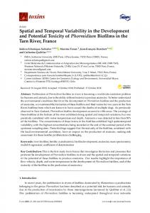
Fig. 10. Schematic vertical cross-section normal to bedrock strike in karst terrain. After Fanning (1970).

In addition to directly affecting streamflow generation by transmitting water through cavities, the bedrock may also exercise indirect control over streamflow generation. Bedrock may affect water flow in the ,,oil by influencing the shape of the soil mantle in places where there is little, or no, saprolite. Figure 10 is a schematic vertical cross-section normal to strike, through a site with tilted karst carbonate strata. On the West Fork, a similar cross-section might be found on the east slope of the perennial stream valley, parallel to the stream channel; as noted earlier, small outcrops that just break the soil surface can be traced upslope in this area, and there appears to be little, or no, saprolite between the bedrock and overlying Alfisols. Between the edges of the more resistant beds, which outcrop at the ground surface, lie bands of deeper soil covering the ends of the less resistant beds. Thus, differential weathering leads to a pattern in which bands of relatively deep soil alternate with outcrops or bands of shallow soil (the bands being parallel to strike and, on the West

158

D.P. GENEREUX ET AL

Fork, normal to the perennial stream channel). This variability in soil thickness could be partially responsible for the difficulty in locating saturated conditions in the soil, even near the stream bank (saturated conditions may be restricted to the areas of deeper soil much of the time). Such variability in saturated condition, s (and in soil moisture in general) could be responsible for some of the observed spatial variability in stream inflow since, other factors being equal, bands of deeper, wetter soil would be associated with stream reaches of higher inflow. This is one restricted sense in which variability in soil thickness (and, therefore, in maximum potential transmissivity) could be partially responsible for the spatial variability in streamflow generation. WBI20-WBI00 is an example of a reach where this phenomenon may be at work. This reach has significantly higher inflow than the adjacent reaches (Fig. 4) and there are rock outcrops which can be traced upslope from the stream channel at approximately WBI20 and WB90. A well point was driven to a depth of 1.5 m about 2 m from the stream bank on the east slope, at WB110; the well was used for groundwater sampling, and yielded water year-round. Attempts at driving well points a few meters upstream and downstream met with refusal at < 1 m, in the unsaturated zone. Thus, this reach of 'locally' high inflow is centered on a band of relatively deep soil (on at least the east slope) which is perennially saturated below 1.5 m and which thins towards the outcrops that lie on either side. A third way (one which operates on all watersheds) in which bedrock geology can affect streamfiow generation is through its influence on topography. Some beds are more erodable than others because of differences in lithology (e.g. on the West Fork, lower chert content) and/or structure (e.g. greater density of fractures), and these beds weather more deeply to produce convergent, hollow-shaped topography. Springs $3 and S3A and their environs (WB242-WB170) provide an interesting example of the relationships among erodability, topography and water flux to the study stream. For reasons discussed in the previous section, the association between high water inflow to this reach and adjacent convergent topography is not due to convergent drainage from the soil mantle (the process responsible at the study site of Anderson and Burt (1978)). Instead, three independent lines of evidence (steady water flow, chemical and temperature characteristics and general lack of a significant soil saturated zone) indicate that most of the inflow to WB242-WB170 is from the bedrock groundwater system. Thus, rather than high stream inflow being due to convergent topography, the high inflow and convergent topography are probably both due to a highly fractured, highly erodable zone in the lower Kingsport Formation. There are no direct observations of the bedrock which point to a greater fracture density in the vicinity

SPATIAL AND TEMPORAL VARIABILITY IN STREAMFLOW GENERATION

159

A

i

• _. 0 • 0

• •

• 00 • ,'?-

Fig. 1I. Runoff in centimeters per day as a function of upstream apparent contributing area on t'~e West Fork. Each of the three plots (i.e. each symbol type) represents one of the graphs in Fig.4.

of WB242-WB170. However, this hypothesis does tie together a variety of hydrogeologic observations in a reasonable manner. In a somewhat trivial sense, one could use the water balance data to argue that the West Fork is not a 'representative' basin for this region (clearly, not every basin in a region can receive a net interbasin transfer of 30-40cm year -~). In addition, the West Fork is probably not 'representative' in the m o r e specific sense suggested by Wood et al. (1988). They suggested the existence of a 'Representative Elementary Area' (REA), which 'is strictly analogous to the concept of the Representative Elementary Volume (REV) in porous media'; the REA would be 'a critical area at which implicit continuum assumptions can be used without knowledge of the patterns of parameter values' (Wood et al., 1988, p.31). Using TOPMODEL, Wood et al. (1988) aetermined an approximate REA for Coweeta Watershed by analyzing the way in which storm runoff volume changed with basin size. A similar analysis can be made with our data, though over a more limited spatial scale (30-40 ha, as opposed to roughly 0.1-500 ha). The streamflow at each stream site in Fig. 4 (WB300, WB280, WB260, etc.) was divided by the total size of the area upstream (the total apparent contributing area) to give the streamflow at each site in units of depth per time. These depth per time streamflow rates (or runoff rates) were then plotted against upstream contributing area (Fig. 11), giving the same kind of plot used by Wood et al. (1988) for their simulated total stormflow volumes. During the lowest flow (Qwe~r = 395 1 min-~ ) experiment, runoff increased with apparent contributing area down to WB 170 (the first measurement site downstream of springs $3 and S3A), and was roughly constant from WBI70 to the weir. In general, constant runoff with increasing scale would suggest that a basin size exceeding the REA had been reached. However, data from the higher flow experiments show sharp increases in runoff downstream of WB60, indicating

160

D.P. GENEREUX ET AL.

that measurements do not extend to a spatial scale at which runoff is relatively constant with basin size, and hence the 38.4 ha West Fork should probably not be considered a REA for the region. (Over a larger range of scales from 0.5 to 38.4 ha, Mulholland et al. (1990) found the same general pattern of increasing runoff with increasing apparent contributing area for stormflow on the West Fork.) The REA (if it can be defined for this landscape) is probably significantly larger than ~ 50 ha, the basin size used in this study, and in most field studies of streamflow generation. Though a basin of this size may include all the topographic and surface hydrologic features of the landscape (valley bottoms, ridge tops, hollows, spurs, ephemeral and perennial stream channels), it does not fully sample the bedrock heterogeneity. Thus, while hydrologic processes on the West Fork are probably typical for karst terrain, the West Fork is probably not 'representative' in the particular sense suggested by Wood et al. (1988). While determination of a REA would probably require data at a larger spatial scale than was spanned by this study, the approach described here does suggest one simple way of using field data to investigate the REA concept. SUMMARY

Chemical dilution stream gauging was used to determine the lateral inflow to stream reaches of various sizes (down to 20 m in length) on a 300 m section of a small stream draining the West Fork of Walker Branch Watershed. For reaches of 60-130 m, the relationships between lateral inflow and Qwe~r (streamflow at the basin outlet) were highly linear over a wide range of flow (350 < Qwc~r< 3500 1 min-~). These relationships can be used to estimate the spatial pattern of stream inflow at a given time from a single Qwe~rmeasurement. Tremendous spatial variability was evident at all scales (reaches of 20-130 m); the permeable karst nature of the dolomite bedrock is the dominant control on the observed variability. This control is probably exerted directly, by water movement through the bedrock, and indirectly, through the effects of geology on topography, and the shape and thickness of the soil mantle. Many of the traditional hillslope hydrometric methods which focus solely on measurement of water flux and/or storage in the soil would be of limited utility in this complex hydrogeologic environment. For thi:~ reason, use of natural tracers has been an important part of the research on the West Fork. The present paper has focused on the amount of water entering the study stream at different places and times (strictly speaking, different places and Qwe~rvalues), and a companion paper (Genereux et al., 1993) describes the use of na'ural tracers in partitioning the stream inflow into water drainage from three hydrogeologic reservoirs.

SPATIAL AND TEMPORAL VARIABILITY IN STREAMFLOW GENERATION

161

ACKNOWLEDGEMENTS

The authors are thankful for the assistance provided by several staff scientists and students at Oak Ridge National Laboratory. Michael Huston and David Lietzke provided useful discussions on soils, topography and other aspects of the study site. The fieldwork would not have been possible without the timely help of Amy Rosemond, Bonnie Lu, Amanda Hood and Lisa Au. Bonnie also analyzed all the chloride samples. This work was sponsored by the U.S. Geological Survey (contract no. 14-08-0001-G-1725) and the National Science Foundation (contract no. BCS-8906032). The first author acknowledges his fellowship support from Oak Ridge Associated Universities, as well as support from the Walker Branch Watershed Project funded by the Ecological Research Division, Office of Health and Environmental Research, U.S. Department of Energy, under contract DE-AC05-84OR21400 with Martin Marietta Energy Systems Inc. Publication 3910 of the Environmental Sciences Division, Oak Ridge National Laboratory. REFERENCES Anderson, M.G. and Burt, T.P., 1978. The role of topography in controlling throughflow ger~eration. Earth Surf. Processes, 3:331-344. Crider, D.V., 1981. Structural and stratigraphic effects on geomorphology and groundwater movement in Knox Dolostone Terrain. M.S. Thesis, University of Tennessee, Knoxville, TN. Fanning, D.S., 1970. Cave features: Information concerning the nature and genesis of soils. Soil Sci. Soc. Am. Proc., 34: 98-104. Fanning, D.S. and Fanning, M.C.B., 1989. Soil: Morphology, Genesis, and Classification. John Wiley and Sons, New York. Generaux, D.P. and Hemond, H.F., 1990. Naturally occurring radon-222 as a tracer for streamflow generation, steady state methodology and field example. Water Resour. Res., 26(I 2): 3065-3075. Genereux, D.P., Hemond, H.F. and Mulholland, P.J., 1993. Use of 222Rn and calcium as tracers in a three-end-member mixing model for streamflow generation on the West Fork of Walker Branch Watershed. J. Hydrol., 142:167-21 I. Henderson, G.S., Harris, W.F., Todd, Jr., D.E. and Grizzard, T., 1977. Quantity and chemistry of throughfall as influenced by forest type and season. J. Ecol., 65: 365-374. Huff, D.D., O'Neill, R.V., Emanuel, W.R., Elwood, J.W. and Newbold, J.D., 1982. Flow variability and hillslope hydrology. Earth Surf. Processes Landforms, 7: 91-94. Johnson, D.W., 1989. Site description. In: D.W. Johnson and R.I. van Hook (Editors), Analysis of Biogeochemical Cycling Processes on Walker Branch Watershed. Springer, New York, pp. 6-20. Jones, H.C., 1912. The Electrical Conductivity, Dissociation and Temperature Coefficients of Conductivity from Zero to Sixty-Five Degrees of Aqueous Solutions of a Number of Salts and Organic Acids. Carnegie Institution of Washington, Washington, DC. Ketelle, R.H. and Huff, D.D., 1984. Site characterization of the West Chestnut Ridge site. ORNL/TM-9229, Oak Ridge National Laboratory, Oak Ridge, TN.

162

D.P. GENEREUX ET AL.

Kline, SJ., 1985. The purpose of uncertainty analysis. J. Fluids Eng., 107: 153-160. Lee, S.Y., Kopp, O.C. and Lietzke, D.A., 1984. Mineralogical characterization of West Chestnut Ridge soils. ORNL/TM-9361, Oak Ridge National Laboratory, Oak Ridge, TN. Lietzke, D.A., 1990. Soils of Walker Branch Watershed. ORNL/TM-iI724, Oak Ridge National Laboratory, Oak Ridge, TN. Lietzke, D.A., Ketelle, R.H. and Lee, R.R., 1989. Soils and geomorphology of the East Chestnut Ridge site. ORNL/TM-! 1364, Oak Ridge National Laboratory, Oak Ridge, TN. Luxmoore, R.J. and Huff, D.D., 1989. Water. In: D.W. Johnson and R.I. van Hook (Editors), Analysis of Biogeochemical Cycling Processes in Walker Branch Watershed. Springer, New York, pp. 164-196. Luxmoore, R.J,, Grizzard, T. and Patterson, M.R., 1981. Hydraulic properties of Fullerton cherty silt loam. Soil Sci. Am. J., 45: 692-698. McMaster, W.M., 1967. Hydrologic data for the Oak Ridge area, Tennessee. U.S. Geological Survey Water Supply Paper 1839-N, U.S. Government Printing Office, Washington, DC. Mulholland, P.J., Wilson, G.V. and Jardine, P.M., 1990. Hydrogeochemical response of a forested watershed to storms: Effects of preferential flow along shallow and deep pathways. Water Resour. Res., 26(12): 3021-3036. Odanski, I., 1975. A rational subdivision of scales for atmospheric processes. Bull. Am. Meteorol. Soc., 56(5): 527-53,9. Peters, L.N., Grigal, D.F., Curlin, J.W. and Selvidge, W.J., 1970. Walker Branch Watershed Report: Chemical, physical, and morphological properties of the soils of Walker Branch Watershed. ORNL/TM-2968, Oak Ridge National Laboratory, Oak Ridge, TN. Soil Conservation Service, 1975. Soil taxonomy: A basic system of soil classification for making and interpreting soil surveys. Agriculture llandbook No.436, U.S. Department of Agriculture, Washington, DC. Tennessee Valley Authority (TVA), 1972. Upper Bear Creek Experimental Project: A continuous daily streamflow model. Research Paper No.8, Tennessee Valley Authority, Knoxville, TN. U.S. EPA, 1983. Methods for chemical analysis of water and Wastes. EPA-600/4-79.020 (350. I- I to 350. I-6), Environmental Monitoring and Support Laboratory, Cincinnati, OH. Weast, R.C., 1976. Handbook of Chemistry and Physics, 56th edn., Chemical Rubber Co., Cleveland, OH. Wilson, G.V. and Luxmoore, R.J., 1988. Infiltration, macroporosity, and mesoporosity distributions on two forested watersheds. Soil Sci. Soc. Am. J., 52: 329-335. Wilson, G.V., Alfonsi, J.M. and Jardine, P.M., 1989. Spatial variability of saturated hydraulic conductivity of two forested watersheds. Soil Sci. Soc. Am. J., 53: 679-685. Wilson, G.V., Jardine, P.M., Luxmoore, R.J. and Jones, J.R., 1990. Hydrology of a forested watershed during storm events. Geoderma, 46:119-138. Wood, E.F, Sivapalan, M., Beven, K. and Band, L., 1988. Effects of spatial variability and scale with implications to hydrologic modelling. J. Hydrol., 102: 29-47. Zar, J.H., 1984. Biostatistical Analysis. Prentice-Hail, Englewood Cliffs, NJ. APPENDIX

As described in the 'Methods' section, two different methods were used to calculate streamflow (Q) values:

(1) Method 1: the specific conductivity change at the measurement site

SPATIAL AND TEMPORAL VARIABILITY IN STREAMFLOW GENERATION

163

farthest upstream, (~,'s--~b)l, was converted to a NaCl concentration (CI) using data from Jones (1912). Q at this station was then determined from the equation QI = QoCo/Ci, where Q0 and Co are the injection rate and NaCl concentration, respectively, of the tracer solution. Q values at sites farther downstream (Qj) were calculated using the flow and specific conductivity data at the first site: Qj = Ql(Ts--~]b)l/(]~s--~b)j. (2) Method 2: the chloride content of background and plateau samples (Sb and Ss, respectively) was measured in the laboratory, and streamflow values were calculated from the expression Qj = QoCo/(Ss--Sb)j. Uncertainty in Qo and Co is directly relevant for both methods. Q0 was measured in the field by capturing the flow from the Mariotte bottle in a graduated cylinder for a period of time (20-30 s) measured with a stopwatch; replicate measurements were always nearly (and often exactly) identical. The flow from a properly functioning Mariotte bottle is extremely steady, and replicate measurements sufficed to establish Q0 to within ,~ 1% (all the uncertainties mentioned in this section refer to 95%, ,~ 2o-, confidence limits). So was determined from the known weights of reagent grade NaC1 ( > 99% pure) and distilled water used to prepare the tracer solution. The mass of NaCl (ms) was determined by weighing out 3-4 aliquots of NaCl (each up to 2500 g, weighed to the nearest 0.2 g); the uncertainty in rnSwas negligible (much less than 1%). The NaCl was placed in a 50 1 carboy, and the carboy was then weighed on a balance with a 50 g resolution. The carboy was filled with distilled water and reweighed on the same balance, and the amount of water (row) was determined by difference. The mass of water was generally about 40 kg, plus or minus about 100 g. The parameter A, defined as 100 mJ(m~ +mw), was calculated for the tracer solution. A linear regression of M (molarity, moles NaC1 per liter of solution) vs. A was calculated using nine data points from Weast (1976, p.D-253) between A = 12 and A = 17 (tracer solutions had A values of 14-15). The resultant straight line (with a correlation coefficient of 0.999949) was used to convert the A value for each tracer solution to a molarity. The uncertainty in the final molarity was very small, about 0.01 M ( < 1%). Thus, the uncertainty in Q0 and Co introduced a negligible uncertainty in the measured streamflow values. The uncertainty associated with streamwater tracer concentrations (explored below for both methods of calculating Q) accounted for most of the uncertainty in the streamflow values.

Method 1 The uncertainty in 7s - ~b values was generally _ 0.4-2/~S cm- ~; the larger uncertainties were obtained when there was significant 7b drift, and when 7b and/or 7s were >/200/zS cm-t (~, values in this range could only be measured

164

D.P. GENEREUX ET AL.

with a resolution of -I-1/~S cm -~, instead of the _ 0.1/~S cm -~ resolution obtained for lower values). Using data from Jones (1912), 0's--~b)~, (the ~s--)'b value at the site farthest upstream) was converted to an equivalent NaCI concentration (C~). Standard statistical methods (Zar, 1984, p.275, equation 17.28) were used to estimate the uncertainty in C~ (it was _ 0.04-0.06 mmol 1-~, depending on the value of C~). The uncertainties in Q0, Co and C~ were propagated according to equation B.4 of Kline (1985) to determine the uncertainty in Q~; this uncertainty, along with those of (~'s- ~b)~ and (~s -- ~b)j, was propagated to determine the uncertainty in other streamflow values (Qj). Total uncertainty in streamflow values calculated by Method 1 averaged 5%, and ranged from 1-11%.

Method 2 The uncertainty in Ss - Sb values was a function of the number of replicate samples and their variability, and the uncertainty in the calibration line on the TRAACS 800 auto analyzer. Usually, three to four samples were collected at ~teady state, one to two at background. The number of steady-state samples was greater because S~ was generally much greater than Sb (0.5-5.0 mmol 1-t, compared with 0.02 mmol 1- ~), hence the uncertainty in S~ - Sb was controlled by uncertainty in Ss (the fact that Sb might be 0.02 + 25-51)% was relatively unimportant). Calibration lines were prepared by running five NaCI standards on the TRAACS 800" the standards had concentrations of 2, 4, 6, 8 and 10 mg 1-t of NaC1 (0.0564-0.282 mmol 1-~ CI-). As noted earlier, & samples were diluted with doubly distilled water to bring their CI- concentrations into the range spanned by the standards. The average uncertainty in S~--Sb values was 6% (the range was 2-17%), leading to an average uncertainty of 7% (the range was 2-18%) in streamflow values determined by Method 2.

Lateral inflow The lateral inflow to a given reach was generally much less than the streamflow at either end of the reach; as a result, a small relative uncertainty in the streamflow values led to a much larger relative uncertainty in lateral inflow. For example, if the lateral inflow to a reach is 10% of the streamflow at the upstream end, and the streamflow at each end has an uncertainty of __5%, the lateral inflow would have an uncertainty of ___74%. Thus, there is a trade-off between spatial resolution and relative uncertainty, with the choice of reach length being determined largely by the intended use of the data. While there is a large relative uncertainty in the lateral inflow to the short reaches

165

SPATIAL AND TEMPORAL VARIABILITY IN STREAMFLOW GENERATION

TABLE A1 Lateral inflow 95% confidence limits for three reaches of the study stream (no measurements were made at WB60 on 4 October 1989; the value given in brackets is for WBI20-WB0) Q,,.~ir (1 min- t )

Lateral inflow (1 min - 1) WB300-WB ! 70

354 395 411 680 709 722 1050 1148 1368 1447 2749 3457

2 4 2 _ !! (4.5%) 281 +___15 (~ 2Yo) 234 + 11 (4.6%) 286 + 20 (7.0%) 346 + 22 (6.3%) 306 + 23 (7.7%) 350 + 21 (6.1%) 375 _____53 (14%) 364 + 38 (10%) 428 + 40 (9.3%) 445 + 123 (28%) 591 + 122 (21%)

WB170-WB60

WB60-WBO

68 3,6 36 67 ,67 91 92 79

+ 17 (24%) 21 + 19(91%) + 22 (63%) 26 +__ 20 (76%) __ 16 (43%) 78 + 20 (26%) + 31 (47%) 166 + 36 (22%) + 34 (51%) 138 + 38 (28%) + 47 (51%) 150 + 50 (33%) _____40 (41%) 260 + 54 (21%) + 74 (94%) 326 + 72 (22%) (482 + 89 (18%)) 109 + 62 (57%) 403 + 76 (19%) 179 + 179 (100%) 1081 __ 267 (25%) 212 +___159 (75%) 1007 _____175 (17%)

shown in Fig. 4 (+50-100%, except for WB220-WBI70 and WB60-WB0), these data are useful in demonstrating the general soatial pattern of stream inflow and the extent of variability. Aggregating the data to larger reaches allowed development of highly linear correlations with Qwe~r(see Fig. 6) which can be used in a predictive mode over a wide range of flows. Table A I gives lateral inflow and uncertainty data for three of ~he reaches shown in Fig. 6. The uncertainty in WB60-WB0 inflow was calculated assuming a 4% uncertainty in Qw~r measurements. The relative uncertainties cover a much wider range than the absolute uncertainties, from 5-10% for much of the WB300WB 170 data to over 90% for some of the very small lateral inflows to the other two reaches. The highly uncertain values represent small differences between two much larger numbers (e.g. the 79 I min-1 value in the eighth row of the WB170-WB60 column is the difference between 822 and 743 1 min -1 ). There were very small decreases in streamflow during most of the experiments; the maximum rate of decrease in Qwe~r(1 1 m i n :) was observed during the highest flow experiment (18 March 1990; average Qwe~rduring the 2 h experiment was 3457 1 min-'). The magnitude of the change in lateral inflow to a given reach can be estimated with the linear regressions in Fig. 6 and the observed rate of decrease in Qweir. For example, the slope of the lateral inflow vs. Qw~ir regression for WB60-WB0 indicates that any change in Qw:~r is associated with a change 36% as large in the lateral inflow to this reach. Thus, the WB60-WB0 lateral inflow would have been decreasing at about

166

D.P. GENEREUX ET AL.

0.36 1 min -2 during the 18 March 1990 experiment, leading to a drop in the lateral inflow rate of 38 1min-~ during the 105 min experiment. This decrease of 38 1 min -~ in the lateral inflow rate of ~ 1000 1 min -~ represents a change of 3.8%. This is much smaller than the lateral inflow uncertainty which ~s due to uncertainty in streamwater tracer concentrations ( + 17% for this reach during this experiment), and unsteadiness in lateral inflow was even less important for other reaches and other experiments. Thus, ignoring the slightly unsteady nature of the stream inflow during our experiments introduces only a very small error which is dwarfed by the uncertainty in the tracer measurements.