Proceedings of the 41st Hawaii International Conference on System Sciences - 2008
Spatial Arbitrage to Reduce “Seams” Across Electricity System Control Areas: An Experimental Analysis* Richard E. Schuler Department of Economics and School of Civil and Environmental Engineering Cornell University
[email protected] (Research Team: Nodir Adilov, Thomas Light, Doug Mitarotonda, Tim Mount, William Schulze, and Ray Zimmerman)
Abstract Most markets are restricted in their spatial size by transportation costs, physical barriers, institutional impediments and differing exchange conventions. Yet, if price differences across those boundaries substantially exceed the cost of surmounting the barriers, tremendous pressure arises to facilitate exchange. So too where electricity markets are defined by operating control areas for reliability purposes, substantial price differences across tie-lines offer incentives for trade and profit. An arbitrage process is developed and tested experimentally that permits buyers and sellers to exchange power across the border of two separately optimized control areas, and the impact on price differences and the ability to exercise market power are explored. While economic efficiency is enhanced and the combined areas are shown to be more competitive than without exchange; nevertheless, the experimental results fall short of the theoretical economic ideal, participant learning is slow, and perverse price patterns (flow from high to low cost control areas) remain in many periods.*
1. Introduction A key attribute that determines the borders of segmented markets is the existence of a physical or institutional barrier. In many instances, these impediments can be reduced by additional expenditures. Thus, a congested transportation network can always be
_____________________________________ *
This work was sponsored by the Power Systems Engineering Research Center (PSERC) and the Consortium for Electricity Reliability Technology Solutions (CERTS). The support provided by PSERC’s industrial members, by the National Science Foundation’s Industry/University Cooperative Research Program under grant NSF EEC-0118300, and by CERTS, supported by the United States Department of Energy is greatly appreciated.
improved by building more facilities (e.g. roads, terminals, or transmission lines, etc.), and a price difference across the boundary provides a clear signal of the benefits to be derived by reducing that congestion. But, the market boundary needs to be specified at the point of congestion. Similarly, if for managerial and reliable operational purposes, the entire U.S. is not operated as a single power grid, then it may make sense to have separate markets in each operating jurisdiction, and to the extent that price differences exist across those “seams”, they may be warranted, in part, by added internal congestion costs that might result from attempts to arrange large transfers across those boundaries (See Adilov and Schuler, 2006, for an overview of these market design considerations). But, to the extent that those price differences exist, they provide powerful incentives to make the arrangements and investments to reduce those physical, financial, and operational procedure barriers. Another consideration in designing the size of a market is to minimize the cost of arbitrage across borders, so it is important to explore the offsetting gains from trade that might be available. Inhibitions to exchange may exist because of a lack of information, different operating rules, or tie-line congestion. In fact, since electricity flows according to the laws of physics, not of commerce, the actual commodity may not flow in the direction or over the path in which an exchange has been negotiated, and more or less congestion may be experienced than anticipated by the traders. This is another reason why electricity traders have been so keen to eliminate rate “pancaking” (charging for transmission access by each jurisdiction across which a contract is negotiated, including adding charges for a reverse flow) when the wholesale markets for electricity were deregulated. Actual flows might not occur over lines for which access fees were paid. However, in practice even with the elimination of rate “pancaking” and in the presence of arbitrage at the borders, some perverse flow continues to be observed where electricity flows from high to low-priced areas (see Holahan and Schuler,
1530-1605/08 $25.00 © 2008 IEEE
1
Proceedings of the 41st Hawaii International Conference on System Sciences - 2008
1988, for a discussion of cases where perverse price patterns may be efficient). The experimental analysis described here is designed to explore the practical possibility of reducing these seams.
2. A Simulated Spatial Market Structure for Electricity 2.1 Physical System Consider two simulated IEEE thirty-bus electricity networks, each with six generator locations, that are connected by a single tie-line between two additional busses, numbers 31 in Region A and number 11 in Region B, as illustrated in Figure 1. Customers may be sited at any of the thirty locations in each simulated network. This combined network is calibrated (details of the calibration are provided in the Appendix) for this exercise with demand and individual generator cost characteristics so that in isolation, the demand and the generation costs are higher in Region B, as compared to Region A. In particular generators 1 and 2 in Region A have the lowest production costs, and generators 5 and 6 in the high demand Region B have the highest costs. Thus, with the connection of the tie-line between Regions A and B, we would expect the predominant flow of electricity to be from A to B. However, by placing the generators with the largest cost differentials at the extreme opposite ends of each region, and allowing for the possibility that lines within each region may become congested as more energy is attempted to be pushed across regions, then that within-region congestion may place severe limits on the actual transfer of power across regions. This type of complication is not unusual on power networks where line flows may be constrained because of thermal or voltage limits on connecting lines.
Tie Line
Note:
(1) Demand Region A < Demand Region B (2) Avg. Production Cost Region A < Avg. Production Cost Region B . 1&2 Lowest Cost) . 5&6 Highest Cost) (Gens (Gens
Figure 1. System Model, Two ISO/RTO Electricity Network
2.2 Generator Dispatch and Market Clearing
Using this simulated electrical network, the normal operation of the system and its economic consequences can be tested under various circumstances. Normally, a system operator in each control area (ISO) arranges the offer curves (price and quantity) of each generator in ascending order in each market period and accepts sufficient offers to ensure that demand is met. Unless supply equals demand in real time, the entire electric system will collapse since large-scale storage is economically infeasible. Furthermore, since these markets are repeated many times per year, it has been shown in other experimental work that for repeated, multi-unit auctions, paying all accepted generators the uniform, last accepted offer leads to the most efficient overall market outcome (see Bernard, et. al., 1998, for an experimental illustration ). As an example, the populist proposal of not paying any supplier more than the price they offer into the market simply causes all suppliers to estimate the market clearing price and to raise their offers to that uniformly high level; whereas with a uniform price being paid to all suppliers based upon the last accepted offer, no infra-marginal supplier has the incentive to raise their offer prices above their costs. The exception may be the generator who thinks they might be the last one selected and therefore capable of setting the market price with her offer.
2.3 Scenarios to be Examined The experimental structure is designed to test the effectiveness of the tie-line and various market structures to facilitate exchange across it in improving overall economic efficiency. Since each generating company owns the generators at two sites, each control area has only three competitive suppliers so these experiments can also demonstrate the effect of a tie-line on the ability to exercise market power. Three benchmarks for optimality are examined: the average prices paid by customers, consumers’ surplus, and producers’ profits. In the first scenario, each region’s system operator minimizes its own total cost of supplying its own customers’ demand. These demand schedules vary between normal and high demand periods and are subject to further random fluctuations. Generation costs are derived from the offers of each supplier in its own region, and the cost minimization is subject to satisfying all reliability criteria. In the second scenario the two regions are connected with a tie line, and the welfaremaximizing solution for both regions, combined, is computed, subject to all of the constraints listed above, as if the combined regions could be operated as an integrated control area. The third set of scenarios recognize the political and physical operational realities that usually make this type of global economic dispatch impossible, in part due to limitations in existing
2
Proceedings of the 41st Hawaii International Conference on System Sciences - 2008
computational technologies that do not permit a timely global solution. In this scenario, both a predetermined bilateral contract for firm transfers, and a market-based set of arbitrage rules are developed and tested against the theoretical, globally optimal benchmarks. In these last two cases, each ISO performs its own locally-optimized dispatch, subject to the exchanges accepted across the tie line through bilateral contracts and/or the arbitrage market. In one case, the arbitrage market is overlaid upon predetermined bilateral commitments to explore whether bi-lateral inefficiencies can be reduced by arbitrage.
2.4 Structure of the Arbitrage Market Each arbitrager chooses the quantity she wishes to transfer from one region to the next, and the direction. She receives or pays that quantity times the actual realized price spread. Since there is no guarantee that the total quantity of energy that arbitragers wish to transfer is within the tie-line capacity, the arbitragers also specify the maximum per MW charge they are willing to pay for their bid to be accepted in the case where the line flow is constrained. This methodology is identical to the economist’s theoretical ideal for pricing services provided from a fixed capital investment (the classic bridge-pricing problem). If the facility is not congested, then going forward the short run marginal cost of permitting another customer to use the facility is zero, since no other customer is inconvenienced. When, however, the usage is sufficient to cause congestion, each additional user inflicts an externality on every other user, and so all customers should be assessed a congestion charge in order to sort out usage priorities efficiently. Furthermore, as those congestion charges rise, they provide an excellent guide to when the construction of additional capacity is warranted. But collecting usage fees merely to cover the capital costs of a project, while essential if the project is arranged and managed by the private sector, is inefficient as a general practice in a social welfaremaximizing sense. In the cross-border markets analyzed here, if a prearranged bilateral contract is in place, its magnitude is added to the transactions scheduled through the arbitrage process. If the capacity constraint is reached, the bilateral contract is always accepted before the arbitragers’ bids. Bilateral contract holders are therefore given priority, as has been common practice in this industry, and they are not assessed congestion charges on the tie-line.
2.5 Calibration of Cost, Demand and Line Constraint Parameters. Values were assigned to each of the system parameters in order to induce electricity flows from Region A to Region B in a majority of periods.
Furthermore, the tie-line capacity was set at 50 Mw and the bilateral contract was set for 25 Mw of firm capacity so that when combined with other parameters in periods with the bilateral contract for transfers in force, perverse flows of electricity from high- to a lower-priced input bus in the adjacent region would be observed. Thus the systems were calibrated to be able to test whether or not the addition of an arbitrage market on top of bilateral contracts would eliminate the perverse flows and improve overall economic efficiency. Calibration details are provided in the Appendix. The potential benefits to be gained by overlaying an arbitrage market were identified in the numerical simulation process that was used to calibrate the system. In simulations where only bilateral contracts govern transfers across the tie-lines, a contract between low-cost generators 1 and 2 in Region A to sell to customers located in the portion of Region B where high cost generators 5 and 6 are located normally increases overall economic efficiency. However, if the within region transmission lines become congested when moving power to and from the borders, perverse pricing patterns between nodes 31 and 11 can occur. If, however, the proper within ISO-congestion charges are assigned to these bilateral transfers, those contracts always proved to be uneconomical in our numerical simulations during conditions when perverse flows developed across the border. Thus an important consequence of adding an arbitrage market may be to permit the adjustment of transfer quantities in periods when those bilateral contracts turn out to be uneconomic, and the prior knowledge that spot market arbitrage is available may enhance the willingness of parties to invest in firm contracts.
3. Description of Experiments on Spatial Arbitrage The six cases (treatments) explored and compared with the results from a theoretically optimal combined dispatch for both ISOs are as follows: 3 Sellers in Each Region (Groups 1 and 2): •
Treatment 1: No Arbitrage/No Power Flow on Tie-line
•
Treatment 2: Arbitrage is Allowed/No PreScheduled Transfer
•
Treatment 3: No Arbitrage/25 MW PreScheduled Transfer from A to B
•
Treatment 4: Arbitrage is Allowed/25 MW PreScheduled Transfer from A to B 6 Sellers in Each Region (Group 3 and 4):
3
Proceedings of the 41st Hawaii International Conference on System Sciences - 2008
•
Treatment 5: No Arbitrage/No Power Flow on Tie-line
•
Treatment 6: Arbitrage is Allowed/No PreScheduled Transfer
Each treatment was conducted for 16 periods during which participants who were graduate students enrolled in a power systems seminar, and therefore were familiar with the operation and markets for electricity, accrued earning in the experiment proportional to their earnings from selling power, including in some treatments, arbitraging across the border. Participants made offers to sell power through the PowerWeb 30 bus simulated electric power grid shown in Figure 1. In treatments where arbitraging was possible, participants also entered their offers to transfer power between regions in an interface designed in Excel that works interactively with Power Web via a market administrator. Each treatment was tested twice with different groups of students. Groups 1, 2 and 3 were comprised of students from October 2005 sessions while group 4’s exercises were conducted in May, 2006. Since fewer participants than required to staff all positions volunteered in May, two positions were played by computer-simulated agents that submitted marginal cost offers for generation and did not participate in arbitrage activities. All arbitrage positions were filled by humans.
3.1 Assumed Ownership Roles and Welfare Accounting Each of the market participant groups and their welfare accounting is described according to the following notation: •
ptA and ptB are the Locational Marginal Prices (LMP) at the tie-line ends in period t in region A and B respectively;
•
Tt ∈[−K, K ] is the net tie-line flow from region A to B. K is the tie-line capacity;
•
λt is the net revenue generated from the tie-line capacity congestion charge in period t;
•
pi,tA and pi,tB are the LMPs for generator i in region A and B respectively in period t;
•
qi,tA and qi,tB are the dispatched quantities for generator i in region A and B respectively in period t;
•
ci,tA and ci,tB are generator i’s total operating costing in period t in region A and B respectively;
•
τ tA
and τ t are the consumer prices of electricity at time t in regions A and B respectively;
•
dtA and dtB are the consumer demand (Mws)
B
at time t in regions A and B respectively; •
I tA and I tB are the imports (in Mws) in period t in regions A and B respectively that are brought in from outside regions A and B, if needed, to meet generation requirements;
• When
dtB ≈
p is the cost/MW of imports. losses i
are
small,
dtA ≈
i
qi,tA − Tt
and
qi,tB + Tt . On average, total losses average
around 2.5 percent of system load.
3.2 Independent System Operators (ISOs) ISO A and B are responsible for determining the least cost dispatch of generators in their own service territory, taking demand and the tie-line flow as given. Each ISO has the potential to collect revenue from its consumers and from flows of power exiting their service territory via the tie-line. The revenue for tie-line flows are presumed to be collected from the Arbitrage Market Administrator. Offsetting these revenues are costs associated with payments to generators and payments to the Arbitrage Market Administrator for flows into the region over the tie-line. Each generator is assumed to receive his LMP on each MW that he is called upon to generate by the ISO. The ISO is required to pay the LMP at the tie-line for any tie-line flows leading into their service territory and will be compensated at the LMP rate for any exiting flows. Consumers are assumed to pay a flat cost/MWh to the ISO regardless of location. The consumer price in each region in each period is calculated as: A t
τ =
i
τ =
i
B t
pi,tA qi,tA − ptATt + pItA dtA pi,tB qi,tB + ptBTt + pItB dtB
,
.
Under this consumer price setting scheme, each ISO runs a balanced budget in every period.
4
Proceedings of the 41st Hawaii International Conference on System Sciences - 2008
Table 2. Average Consumer Price ( τ t and τ t ) by Treatment A
3.3 Arbitrage Market Administrator (AMA) The AMA is responsible for clearing the tie-line arbitrage market, facilitating the transfer of power between regions, and imposing a tie-line capacity congestion charge (credit) when the requested net flow exceeds the tie-line capacity. In order to do this, it collects offers from arbitragers and in treatments 3 and 4 also takes as given the 25 MW pre-scheduled flow over the tie-line. In the process of clearing the market, the AMA is responsible for purchasing and selling power in the respective ISOs depending on the direction of the tieline flow. The AMA runs a balanced budget in periods where the tie-line flow is less than the tie-line capacity and runs a positive budget of λt in periods where the tieline is loaded to capacity. Table 1. Average Congestion Value Treatment
λt by
Average Capacity Limit Congestion Charge Revenue NA $60.92
Treatment 1 Treatment 2 Treatment 3 Treatment 4
NA $6.73
Treatment 5 Treatment 6
NA $20.35
Social Optimum
$0.00
Table 1 reports the average value of λt for each treatment. In general, the AMA runs a small positive budget in the treatments which allow arbitrage. These revenues could presumably be put towards maintaining the tie-line.
3.4 Consumers In every treatment, demand is stochastic but unresponsive to real time power costs. Consumer welfare in each region will therefore vary with the aggregate consumer cost of power in regions A and B, calculated as dt τ t and dt τ t , respectively. Therefore, consumers in each region will be made better or worse off depending on the cost of power. As a result, A
A
B
B
consumer prices, τ t and τ t , are the measures of consumer welfare for each treatment. A
B
B
Average Consumer Price per MW Region A Region B Combined $74.72 $89.04 $82.37 $56.03 $81.46 $69.61
Treatment 1 Treatment 2 Treatment 3 Treatment 4
$85.61 $78.54
$99.60 $100.26
$93.06 $90.14
Treatment 5 Treatment 6
$46.56 $42.32
$71.88 $67.11
$60.09 $55.56
Social Optimum
$39.89
$52.89
$46.87
Table 2 shows the average consumer price/MW after pooling the results across groups. It suggests that the introduction of the arbitrage market generally reduces consumer prices in both regions.
3.5 Generators Aggregate generator profits in each of the respective regions are calculated as:
π tA =
i
pi,tA qi,tA − ci,tA ,
π tB =
i
pi,tB qi,tB − ci,tB .
Table 3. Average Generator Profits ( π t and Per Period by Region and Treatment A
Treatment 1 Treatment 2
π tB )
Average Aggregate Generator Profits per Period Region A Region B Combined $7,043 $8,192 $15,236 $4,677 $6,308 $10,985
Treatment 3 Treatment 4
$10,331 $8,723
$8,967 $9,436
$19,298 $18,159
Treatment 5 Treatment 6
$1,767 $2,108
$4,491 $3,713
$6,258 $5,821
Social Optimum
$1,018
$1,027
$2,045
Table 3 reports the average total generator profits per period in each region separately, and combined, for each treatment. In most cases those profits are lower with arbitrage across the tie-line because the market is more competitive.
3.6 Arbitragers Arbitragers make money depending on the direction of their accepted transfer, the tie-line border prices, and any capacity congestion charge (or credit) levied.
5
Proceedings of the 41st Hawaii International Conference on System Sciences - 2008
Aggregate arbitrager earnings can therefore be calculated as
ψ t = ( p − p )Tt − λt B t
A t
in periods where no bilateral is in place and
ψ t = ( ptB − ptA )(Tt − 25) − λt in treatments when the 25 MW bilateral contract is in effect. Table 4 shows the average total arbitrager earnings per period by treatment. On average, arbitragers lost money in every treatment. The losses from arbitrage activities were greatest in treatments 5 and 6 when the individual ISOs were most competitive. Table 4. Average Total Arbitrage Earnings ( ψ t ) per Period by Treatment Treatment 1 Treatment 2
Average Arbitrager Earnings per Period NA -$476
Treatment 3 Treatment 4
NA -$419
Treatment 5 Treatment 6
NA -$1,246
Social Optimum
$0
3.7 Owner of Pre-Scheduled Bilateral Transfers To keep the analysis simple, the pre-scheduled bilateral transfer is viewed as a financial contract for a 25 MW flow from A to B over the tie-line. The owner of the pre-scheduled bilateral, like the arbitragers, makes or loses money based on the border price differences but is assumed able to avoid paying tie-line capacity congestion charge. As such, the bilateral contract owner will experience profits in treatments 3 and 4 equal to:
ηt = ( p − p )25 . B t
A t
Table 5 reports the average earnings that accrued to the owner of the bilateral contract in each period. Here arbitrage across the tie-line enhances the profitability of a fixed bi-lateral contract. Table 5. Average Bilateral Earnings ( ηt ) per Period Treatment 1 Treatment 2
Average Bilateral Earnings per Period NA NA
Treatment 3 Treatment 4
$39 $196
Treatment 5 Treatment 6
NA NA
Social Optimum
$0
3.8 Total Welfare A measure of total welfare can be calculated by adding together the participant group welfare measures described above. Formally, we add together: 1. ISO A and B Welfare: 0 (due to budget balance consumer pricing condition). 2. Arbitrage Market Administrator: λt (only when arbitraging is allowed).
τ tA − dtBτ tB . A B Generator Surplus: π t + π t . Arbitrager Surplus: ψ t (only when
3. Consumer Surplus: − dt
A
4.
5. arbitraging is allowed). 6. Bilateral Contract Holder: ηt (only when bilateral is in place). The addition of the welfare measures shows that aggregate social welfare is maximized when the aggregate cost of production in both regions is minimized:
c +
A i i,t
c + pI tA + pI tB .
B i i,t
This is due to the fact that demand is perfectly inelastic, and all market activities other than power production only shift welfare between participant groups. Table 6 provides the average cost of power production per period for each treatment. Table 6. Average Cost of Power Production per Period (
Treatment 1 Treatment 2
c +
A i i,t
c + pI tA + pI tB )
B i i,t
Average Cost of Power Production per Period Region A Region B Combined $7,298 $11,536 $18,834 $8,290 $11,329 $19,619
Treatment 3 Treatment 4
$8,700 $8,676
$10,439 $10,712
$19,138 $19,388
Treatment 5 Treatment 6
$7,192 $7,515
$11,341 $11,684
$18,533 $19,199
Social Optimum
$7,408
$9,762
$17,170
Table 6 suggests that the even numbered treatments that involve the arbitrage market (2,4 and 6) always perform worse in terms of aggregate social welfare. A partial explanation for this might be that the arbitrage introduces more uncertainty for generators, causing a greater proportion of production to come from expensive imports. Table 7 shows the average Mw imported each period for each of the treatments.
6
Proceedings of the 41st Hawaii International Conference on System Sciences - 2008
Table 7. Average Imports by Treatments Treatment 1 Treatment 2
Average MW Imported Per Period Region A Region B Combined 0.25 1.38 1.62 11.64 2.43 14.07
Treatment 3 Treatment 4
1.78 0.93
0.00 1.75
1.79 2.68
Treatment 5 Treatment 6
0.36 8.09
0.24 0.42
0.60 8.51
-
-
-
Social Optimum
This result is statistically significant except in region A under treatment 6. •
Imports are assumed to cost $110/MW which is about twice as much as the incremental cost of the most expensive internal generator.
Impact of Introducing the Arbitrage Market: A comparison of treatments 1 with 2, 3 with 4, and 5 with 6 provides mixed results. o
When comparing treatments 1 and 2, consumers were better off in both regions after introducing the arbitrage market. This finding is statistically significant at the 99 percent level in region A and for the combined markets, and at the 96 percent significance level in region B.
o
When comparing treatments 3 with 4, we find that consumers in region A are made better off. The treatment effect for 3 and 4 are not statistically different from one another in region B or both regions combined, however.
o
A comparison of treatments 5 and 6 suggest that consumers in both regions are made better off from the arbitrage market. This result is only statistically significant when looking at the combined consumer surplus for both regions, however.
4. Statistical Tests of Market Design Effects on Welfare and Efficiency Regressions were run to measures the effect of different market treatments on consumer, producer, and total welfare. The regression specification includes group specific demand effects as well as treatment effects. A chi-squared test was performed of the null hypothesis that treatment effects are equal for each regression. Thus a rejection of the hypothesis implies that the outcomes between treatments are significantly different. The regressions include 16 observations for each treatment experienced by each of the four groups, plus, as the base case, 16 observations for each group representing outcomes that would be obtained in the economist’s perfectly competitive world with efficient transfers between the regions (equivalent to the social optimum). In total there are 256 observation used for each regression. In addition to these welfare measures, the analysis also investigates the effect of different market structures on price differences at either end of the tie-line. Under an efficiently operating arbitrage market, these border prices would be equal.
4.1 Consumer Welfare: Consumer Cost per Mw (Table 2) Regressions were run on the average consumer price of power in each region for each period, as well the quantity-weighted average consumer cost of power across both regions. The regressions control for the demand state and individual group effects. A summary of the results is: •
Comparison with Social Optimum: In all treatments, consumers were statistically worse off than they would be at the social optimum.
•
Impact of Allowing Bilateral Contracts without Allowing for Arbitraging: Comparing treatments 1 and 3 suggests that bilateral contracts make consumers worse off in all regions with high statistical significance.
•
Impact of Introducing More Competition in Both Regions: Comparing treatments 1 with 5 and 2 with 6, consumers are made better off in both regions when the number of generators is doubled from 3 to 6 in each region. This result holds with high statistical significance in all cases.
•
Impact of Introducing Both Bilateral Contracts Comparing and the Arbitrage Market: treatments 1 and 4 suggests that consumers would not be made better off by introducing both bilateral contracts and the arbitrage market.
4.2 Producer Welfare (Table 3) The regression analysis measures how each of the treatments affects generator profits, after controlling for group and forecast demand effects. In a second set of regressions, arbitrage earnings were added to producer earnings and the analysis for both regions combined was
7
Proceedings of the 41st Hawaii International Conference on System Sciences - 2008
repeated. In the latter regression the effect of participant learning was also tested. The key findings concerning producer surplus are: •
•
Comparison with Social Optimum: Producers earned statistically significantly more than they would in the social optimum under every treatment. Impact of Introducing the Arbitrage Market: Comparing treatments 1 with 2, 3 with 4, and 5 with 6, as with the consumer surplus tests, yielded mixed results. o
•
•
When comparing treatments 1 and 2, producers are always made worse off when the arbitrage market is introduced.
o
When comparing treatments 3 with 4, a statistically significant decline in profits is seen in region A but not region B.
o
A comparison of treatments 5 and 6 yields no statistically significant differences.
Impact of Allowing Bilateral Contracts without Allowing for Arbitrage: Comparing treatments 1 and 3, the introduction of bilateral contracts increase seller profits in Region A but not B. This is consistent with the notion that the bilateral contract from A to B should increase the market power in region A and reduce market power in region B. Impact of Introducing More Competition in Both Regions: Comparing treatments 1 with 5 and 2 with 6 shows that producers in aggregate are made worse off in every case when the number of competitors is increased.
•
Impact of Introducing Both Bilateral Contracts and the Arbitrage Market: Comparing treatments 1 and 4, profits increase in treatment 4 relative to 1. This finding is statistically significant in region A but not B.
•
Learning Effects: To test whether participants are learning over the course of each treatment, a time trend was introduced to the regressions that incorporate both producer earnings from power production and arbitrage earnings as the dependent variable. The coefficient on period of play has no statistical significance indicating that learning is not likely to have occurred on a systematic basis within each treatment. There may, however, be learning effects across
treatments, but there is no clear way of testing for this since it is impossible to distinguish learning from the treatment effect.
4.3 Aggregate Social Welfare Aggregate social welfare is maximized when the total cost of power production in both regions is minimized. The aggregate cost of production in both regions by period for each treatment suggests: •
Comparison with Social Optimum: The cost of power production is statistically greater in every treatment, compared with the social optimum.
•
Impact of Introducing the Arbitrage Market: In every case where the arbitrage market is added incrementally (going from treatments 1 to 2, 3 to 4, or 5 to 6), the cost of power production goes up, suggesting that aggregate social welfare declines. This may be explained by noticing that the arbitrage market has a tendency to make the power production requirements in any one region more sporadic. This coupled with the fact that sellers face standby costs, suggests that sellers may have stronger incentive to offer in less capacity in any given period. As a result, the dispatch of sellers is likely to be less efficient when compared with the case where sellers can anticipate with greater precision their ISO’s production requirements.
•
Impact of Allowing Bilateral Contracts without Allowing for Arbitraging: The treatment effect associated with treatments 1 and 3 are not statistically distinguishable from one another, suggesting that the 25 MW bilateral does not have a significant impact on overall welfare in the experiments.
•
Impact of Introducing More Competition in Both Regions: Treatments 1 and 5 and 2 and 6 are statistically indistinguishable suggesting that increasing competition only shifts surplus from producers to consumers without effecting the combined total surplus.
•
Impact of Introducing Both Bilateral Contracts and the Arbitrage Market: Comparing treatments 1 and 4, bilateral contracts in combination with the arbitrage market leads to lower total surplus. This finding holds with 99 percent statistical significance.
4.4 Border Prices In a fully efficient dispatch of generators across regions, the prices at each end of the tie-line connecting
8
Proceedings of the 41st Hawaii International Conference on System Sciences - 2008
regions would be approximately equal if the line is not congested and losses on transfers across the tie-line are minimal. Regressions were run on the absolute value of the price differences at the border where the prices are determined by each ISO independently via their OPF. A comparison of treatment 1 and 2 in Table 8 suggests that the arbitrage market works as expected; namely, it reduces price differences at the border. However, a comparison of treatments 3 with 4 and 5 with 6 suggests that the arbitrage market did not perform as expected in these cases. At the end of treatment 4 it was clear that at least one participant was acting strategically to manipulate the tie-line flow, presumably to improve his earnings from generation.
5.5 Overall Conclusions: Spatial Arbitrage The statistical analysis of the seams experiment suggests the following results: •
Competitive Effects: The introduction of an arbitrage market between control areas has the potential to reduce the system-wide average generator prices and profits. This effect was found to be statistically significant in most cases where generators had initial market power (treatments 1 – 4). The implication is that the introduction of real-time markets for transfers between control areas can improve market conditions by increasing the number of effective competitors. This was shown to benefit consumers by reducing the retail price of electricity in the experiments.
•
Efficiency: While the incorporation of an arbitrage market for flows between ISOs was found to increase competition in many cases, it also had a tendency to increase the average production cost/Mwh experienced by generators. This is at least partially due to increased uncertainty faced by generators for production needs within their service territory brought about by speculative behavior by participants in the arbitrage market. As a result, overall economic efficiency tends to be lower with the arbitrage market in place in these experiments, despite its ability to reduce market power.
Table 8. Border Price Difference Regression (Dependent Variable: Absolute Value of Border Price Difference) Coef.
Std. Err.
Dependent Variable: Absolute Value of Border Price Difference Treatment Treatment Treatment Treatment Treatment Treatment Treatment R-squared Obs
Effects 1 2 3 4 5 6
34.43 23.40 15.80 20.94 13.01 30.87
2.49 2.49 2.49 2.49 2.49 2.49 0.695 256
As an illustration, Figure 2 compares price differences across the border, with and without arbitrage, for one of the experimental groups where there were six generators in each ISO. In many instances, the price gaps were wider with arbitrage, and flow persisted in a perverse direction; although there was some modest improvement over time.
Figure 2. Border Prices and Tie Line Flows (Six Sellers in Each ISO, w and w/o Arbitrage)
Even though the introduction of an arbitrage market on top of a pre-existing bilateral contract across the control areas tended to reduce the frequency of perverse flows on that line, as arbitragers gained experience (see Figure 2), those perverse flows were not eliminated totally. In these experiments the generators were also free to engage in arbitrage across the borders. Their incentive to speculate may have increased as the tie-line became congested, which was more likely with a pre-existing bilateral exchange. •
Reliability: At times, market clearing in the arbitrage market generated large power swings on the tie-line between control areas. In many cases, these swings cannot be attributed to forecast events such as changing demand within each ISO. This suggests that reliability may be compromised by enabling market participants to
9
Proceedings of the 41st Hawaii International Conference on System Sciences - 2008
speculate on flows into or out of their own service territory. •
Distributional Implications: When trading is possible between control areas, one region ends up benefiting at the expense of customers or producers in the neighboring region. As a result, a well-designed market that generates system wide operational and economic efficiencies may not be sufficient to ensure political feasibility.
Appendix: Calibration of the Spatial Experiment Demand and generator costs in each region were calibrated in such a way that the optimal transfer between region A and B varied considerably depending on whether it was a normal or high demand period. For the experiment, the average demand varied between 180 to 200 MW in region A and 200 to 240 MW in region B depending on whether the period was a normal or high demand period respectively. Actual demand varied by an additional 10 percent around the average forecast demand for each type of demand condition. Table A1 reports the generator cost assignments used in treatments 1 through 4. In these treatments, each participant was assigned two generators in either region A or region B. In treatments 5 and 6, the capacity of each generator was divided into two 30 MW blocks with the same variable and standby costs. Participants in treatments 5 and 6 were assigned two 30 MW blocks in either region A or region B, but the blocks were not necessarily located at the same node location. As a result, we would expect more intense competition in treatments 5 and 6. Table A1: Generator Costs Structure Used in Treatments 1 through 4 Generator Variable C it C t/MW
Region A
Standby C t/MW
C
Fixed t/P i d
Generator Generator Generator Generator Generator Generator
1 2 3 4 5 6
60 60 60 60 60 60
$15.00 $25.00 $35.00 $35.00 $45.00 $55.00
$5.00 $5.00 $5.00 $5.00 $5.00 $5.00
$45.00 $45.00 $45.00 $45.00 $45.00 $45.00
Region B Generator Generator Generator Generator Generator Generator
1 2 3 4 5 6
60 60 60 60 60 60
$35.00 $35.00 $35.00 $55.00 $55.00 $55.00
$5.00 $5.00 $5.00 $5.00 $5.00 $5.00
$120.00 $120.00 $120.00 $120.00 $120.00 $120.00
Table A2 shows the resulting power transfers and border prices obtained under marginal cost offers, and under alternative dispatch and transfer assumptions. The results obtained from the combined OPF represent a global social optimum where total generator costs in both regions are minimized. The separate OPF outcomes, with and without a transfer, are representative of what would occur in a highly competitive environment when each region is independently optimized on generation cost. Notice that these results suggest that we would expect a perverse tie-line flow to occur under normal demand conditions when the 25 MW bilateral transfer is present. Table A2: Tie-Line Flows and Border Prices Under Alternative Dispatch Conditions Tie Line Flow From Region A to B (MW)
Average Normal Demand Period Combined OPF Separate OPFs w. 25 MW Transfer Separate OPF w. no Transfer Average High Demand Period Combined OPF Separate OPFs w. 25 MW Transfer Separate OPF w. no Transfer
Border Price Region A
Region B
4.14
$50.00
$50.00
25.00
$50.00
$41.07
0.00
$50.00
$52.97
28.58
$52.02
$52.03
25.00 0.00
$51.63 $50.00
$54.57 $58.09
Note: Assumes all generators make marginal cost offers.
References Adilov, N. And Schuler, R., 2006, “Electricity Markets: How Many, Where and When?”, Symposium on Electric Power Systems Reliability, Control and Markets, Hawaii International Conference on Systems Science 39, Kauai, HI. Bernard, J., Schulze, W.,Mount, T., Zimmerman, R., Thomas, R., and Schuler, R., 1998, “Alternative Auction Institutions for Purchasing Electric Power: An Experimental Examination”, Proceedings of Bulk Power Systems Dynamics and Control IV – Restructuring, Santorini, Greece. Holahan, W.L. and Schuler, R.E. 1988, “Imperfect Competition in a Spatial Economy: Pricing Policies and Economic Welfare,” CORE Discussion Paper 8821, Universite Catholique de Louvain, Louvain-la-Neuve, Belgium, March 1988.
10