Spatial Databases and Geographical Information Systems

zk0

SPATIAL DATABASES AND GEOGRAPHICAL INFORMATION SYSTEMS (GIS)

HANAN SAMET COMPUTER SCIENCE DEPARTMENT AND CENTER FOR AUTOMATION RESEARCH AND INSTITUTE FOR ADVANCED COMPUTER STUDIES UNIVERSITY OF MARYLAND COLLEGE PARK, MARYLAND 20742-3411 USA

Copyright © 2002 Hanan Samet These notes may not be reproduced by any means (mechanical or electronic or any other) without the express written permission of Hanan Samet

zk1 OUTLINE 1. GIS overview 2. Background 3. General database issues 4. Spatial indexing 5. The SAND browser 6. Spatial database issues 7. Challenges

zk2 WHAT IS A GIS? Def: a system that uses spatial (i.e., geographically referenced) and non-spatial (i.e., attribute) data and includes operations that support spatial analysis Alternative names: •

AM/FM (automated

mapping and facilities management)

• geographically referenced information system • land information system • natural resources information system • spatial data management (or handling) system • spatial database

zk3 FIELDS THAT ARE INVOLVED IN GIS 1. Cartography—display of visual information 2. Civil Engineering—transportation 3. Computer science—databases, computer graphics, image processing 4. Geodesy—high accuracy positional control 5. Geography—spatial analysis, relation of man to world 6. Mathematics—geometry, graph theory 7. Operations research—optimization 8. Photogrammetry—aerial photographs are best sources for topography 9. Remote sensing—images from space 10. Statistics—models, analysis of error 11. Surveying—position of land boundaries, buildings, etc.

zk4 SOME TYPICAL GIS QUERIES 1. What feature is at location X ? 2. Does feature F exist anywhere? 3. Report the identity of all features present 4. Select all the locations where feature F is present 5. Where is object A with respect to object B ? 6. Simulate the effect of phenomenon P for time period T in area A 7. What is the cheapest, fastest, or least resistant path from A to B ? 8. What is the value of function f at location X ? 9. What is the result of overlaying a given set of map layers? 10. What is the result of intersecting a given set of map layers? 11. What combination of features is at location X ? 12. Where is object A in relation to object B or location X ? 13. Report all features within distance d of location X or object A 14. Reclassify certain ranges of feature values 15. Proximity queries such as what objects are next to other objects having certain attribute values 16. Measure properties such as area, perimeter, etc.

zk5 GIS OPERATIONS 1. Display the data 2. Find a pattern in the data • knowledge discovery • “what is” or “what could be”? • usually by decomposing data into finer levels of meaning 3. Predict the behavior of the data at another time and place • “what should be”?

zk6 GIS ANALYSIS FUNCTIONS 1. Local operations • retrieval • classification and recoding • generalization—reducing detail • measurement 2. Overlay operations 3. Neighborhood operations • search • proximity—e.g., Voronoi diagrams •

TIN generation

• interpolation • contour generation • buffer or corridor generation 4. Connectivity operations • network functions—e.g., flow, routing, siting • spread functions—i.e., phenomena accumulate with distance • seek or stream functions—e.g., drainage • intervisibility

zk7 EXAMPLE OF GIS (MUNICIPAL DATABASE) 1. Basemap data • control points • topographic contours • building sites 2. Natural area data • soil types • landuse (e.g., industrial, agricultural, zoning, etc.) • vegetation • water (e.g., rivers, ponds, etc.) 3. Manmade area data • school districts • emergency service areas (e.g., fire, police, etc.) 4. Land records data • lot boundaries • zoning • easements and rights-of-way 5. Network data • utilities (e.g., phones, sewers, water, electricity, etc.) • roads a. road centerlines b. road intersections c. street lights

zk8 BACKGROUND (A PERSONAL VIEW!) 1. GIS originally focussed on paper map as output • anything is better than drawing by hand • no great emphasis on execution time 2. Paper output supports high resolution • display screen is of limited resolution • can admit less precise algorithms • Ex: buffer zone computation (spatial range query) a. usually use a Euclidean distance metric (L2) • takes a long time b. can be sped up using a quadtree and a Chessboard distance metric (L∞) • not as accurate as Euclidean — but may not be able to perceive the difference on a display screen! • as much as 3 orders of magnitude faster 3. Users accustomed to spreadsheets • GIS should work like a spreadsheet • fast response time • ability to ask “what if” questions and see the results • incorporate a database for seamless integration of spatial and nonspatial (i.e., attribute data)

zk9 GENERAL SPATIAL DATABASE ISSUES 1. Why do we want a database? • to store data so that it can be retrieved efficiently • should not lose sight of this purpose 2. How to integrate spatial data with nonspatial data 3. Long fields in a relational database are not the answer • a stopgap solution as just a repository for data • does not aid in retrieving the data • if data is large in volume, then breaks down as tuples get very large 4. A database is really a collection of records with fields corresponding to attributes of different types • records are like points in a higher dimensional space a. some adaptations take advantage of this analogy b. however, can act like a straight jacket in case of relational model 5. Retrieval is facilitated by building an index • need to find a way to sort the data • index should be compatible with data being stored • choose an appropriate zero or reference point • need an implicit rather than an explicit index a. impossible to foresee all possible queries in advance b. explicit would sort two-dimensional points on the basis of their distance from a particular point P • impractical as sort is inapplicable to points different from P

zk10 6. Identify the possible queries and find their analogs in conventional databases • e.g., a map in a spatial database is like a relation in a conventional database (also known as spatial relation) a. difference is the presence of spatial attribute(s) b. also presence of spatial output 7. How do we interact with the database? •

SQL

may not be easy to adapt

• graphical query language • output may be visual in which case a browsing capability (e.g., an iterator) is useful 8. What strategy do we use in answering a query that mixes traditional data with nontraditional data? • need query optimization rules • must define selectivity factors a. dependent on whether index exists on nontraditional data b. if no, then select on traditional data first • Ex: find all cities within 100 miles of the Mississippi River with population in excess of 1 million a. spatial selection first if region is small (implies high spatial selectivity) b. relational selection first if very few cities with a large population (implies high relational selectivity)

zk11 DATA IN SPATIAL DATABASES 1. Spatial information • locations of objects (are discrete, individual points in space) • space occupied by objects (are continuous; have extent) a. example objects • lines (e.g., roads, rivers) • regions (e.g., buildings, crop maps, polyhedra) • others ... b. are objects disjoint or may they overlap? • e.g., several crop types may be grown on a plot of land • not concerned here with raster vs: vector issues as these are data representation issues rather than data type issues 2. Non-spatial information • region names, postal codes, ... • city population, year founded, ... • road names, speed limits, ...

zk12 SAMPLE QUERIES ON SPATIAL OBJECTS • Queries about the objects 1. all objects that contain a given point or set of points 2. all objects that have a non-empty intersection with a given object 3. all objects that have a partial boundary in common 4. all objects that have a boundary in common 5. all objects that have any points in common 6. all objects that contain a given object 7. all objects that are included in a given object • Proximity queries 1. nearest object to a given point or object 2. all objects within a given distance of a point or object (also known as a range or window query) • Queries involving non-spatial attributes of objects 1. given a point or object, find the nearest object of a particular type 2. Given a point, find the minimum enclosing object of a particular type 3. Given a point, find all the objects of a particular type whose boundary passes through it

zk13 WHAT MAKES CONTINUOUS SPATIAL DATA DIFFERENT 1. Spatial extent of the objects is the key to the difference 2. A record in a DBMS may be considered as a point in a multidimensional space • a line can be transformed (i.e., represented) as a point in 4-d space with (x1 , y1 , x2 , y2 ) (x2, y2) (x1, y1) • good for queries about the line segments • not good for proximity queries since points outside the object are not mapped into the higher dimensional space • representative points of two objects that are physically close to each other in the original space (e.g., 2-d for lines) may be very far from each other in the higher dimensional space (e.g., 4-d) • Ex: • problem is that the transformation only transforms the space occupied by the objects and not the rest of the space (e.g., the query point)

A B

• can overcome by projecting back to original space 3. Use an index that sorts based upon spatial occupancy (i.e., extent of the objects)

zk14 SORTING ON THE BASIS OF SPATIAL OCCUPANCY • Decompose the space from which the data is drawn into regions called buckets (like hashing but preserves order) • Interested in methods that are designed specifically for the spatial data type being stored • Basic approaches to decomposing space 1. minimum bounding rectangles • e.g., R-tree • good at distinguishing empty and non-empty space • drawbacks: a. non-disjoint decomposition of space • may need to search entire space b. inability to correlate occupied and unoccupied space in two maps 2. disjoint cells • drawback: objects may be reported more than once • uniform grid a. all cells the same size b. drawback: possibility of many sparse cells • adaptive grid — quadtree variants a. regular decomposition b. all cells of width power of 2 • partitions at arbitrary positions a. drawback: not a regular decomposition b. e.g., R+-tree • Can use as approximations in filter/refine query processing strategy

4321 gz r b

zk15

MINIMUM BOUNDING RECTANGLES Objects grouped into hierarchies, stored in another structure such as a B-tree Drawback: not a disjoint decomposition of space Object has single bounding rectangle, yet area that it spans may be included in several bounding rectangles Examples include the R-tree and the R*-tree Order (m,M ) R-tree 1. between m M/2 and M entries in each node except root 2. at least 2 entries in root unless a leaf node R1

R3 b a

R4 h R5 R2

g

R6 e i

d

f

c

R0

R0: R1 R2

R1: R3 R4

R3: a

b

R4: d

R2: R5 R6

g

h

R5: c

i

R6: e

f

54321 gz r vb

SEARCHING FOR A POINT OR LINE SEGMENT IN AN R-TREE

zk16

Drawback is that may have to examine many nodes since a line segment can be contained in the covering rectangles of many nodes yet its record is contained in only one leaf node (e.g., i in R2, R3, R4, and R5) Ex: Search for a line segment containing point Q R0: R1 R2

R1: R3 R4

R3: a

b

R2: R5 R6

g

R4: d

R5: c

h

R1

i

R6: e

f

R3 b a h R6 e

g i d

Q

f

R4 R0

R2

R5

c

Q is in R0 Q can be in both R1 and R2 Searching R1 first means that R4 is searched but this leads to failure even though Q is part of i which is in R4 Searching R2 finds that Q can only be in R5

zk17 UNIFORM GRID Ideal for uniformly distributed data Supports set-theoretic operations Spatial data (e.g., line segment data) is rarely uniformly distributed

zk18 QUADTREES • Hierarchical variable resolution data structure based on regular decomposition • Many different decomposition schemes and applicable to different data types: 1. points 2. lines 3. regions 4. rectangles 5. surfaces 6. volumes 7. higher dimensions including time • changes meaning of nearest a. nearest in time, OR b. nearest in distance • Can handle both raster and vector data as just a spatial index • Shape is usually independent of order of inserting data • Ex: region quadtree • A decomposition into blocks — not necessarily a tree!

zk19 REGION QUADTREE • Repeatedly subdivide until obtain homogeneous region • For a binary image (BLACK ≡ 1 and WHITE ≡ 0) • Can also use for multicolored data (e.g., a landuse class map associating colors with crops) • Can also define the data structure for grayscale images • A collection of maximal blocks of size power of two and placed at predetermined positions 1. could implement as a list of blocks each of which has a unique pair of numbers: • concatenate a sequence of 2 bit codes corresponding to the path from the root to the block’s node • the level of the block’s node 2. does not have to be implemented as a tree • tree good for logarithmic access • A variable resolution data structure in contrast to a pyramid (i.e., a complete quadtree) which is a multiresolution data structure 0 0 0 0 0 0 0 0

0 0 0 0 0 0 0 0

0 0 0 0 0 0

1 1 1 1 1 1

0 0 0 0 0 0

0 0 0 1 1 1

0 0 1 1 1 1

1 1 1 1 1 0

1 1 1 1 0 0

1 1 1 1 0 0

J

37 38 39 40

L

M

B

SE SW

C

D

E

K F

G

H

I

J

P L

37 38 39 40

G

H

I

N

O

57 58 59 60

A NW NE

F B

M

N

O

Q

57 58 59 60

Q

zk20 PYRAMID • Internal nodes contain summary of information in nodes below them • Useful for avoiding inspecting nodes where there could be no relevant information

c1 c2 c3

c4 c5 c6

{c1,c2,c3,c4,c5,c6} {c1,c2,c3, c4,c5,c6} {c6}

{c2,c3,c6}

{c2,c3,c4,c5}

zk21 QUADTREES VS. PYRAMIDS • Quadtrees are good for location-based queries 1. e.g., what is at location x? 2. not good if looking for a particular feature as have to examine every block or location asking “are you the one I am looking for?” • Pyramid is good for feature-based queries — e.g., 1. does wheat exist in region x? • if wheat does not appear at the root node, then impossible to find it in the rest of the structure and the search can cease 2. report all crops in region x — just look at the root 3. select all locations where wheat is grown • only descend a node if there is a possibility that wheat is in one of its four sons — implies little wasted work • Ex: truncated pyramid where 4 identically-colored sons are merged {c1,c2,c3,c4,c5,c6} {c1,c2,c3, c4,c5,c6} {c6}

c1 c2 c3

c4 c5 c6

{c2,c3,c6}

{c2,c3,c5}

{c2,c3,c4,c5}

{c1,c2,c3,c5}

• Can represent as a list of leaf and nonleaf blocks (e.g., as a linear quadtree)

8 7 6 5 4 3 2 1 r z g v g z r b

PR QUADTREE (Orenstein)

zk22

1. Regular decomposition point representation 2. Decomposition occurs whenever a block contains more than one point 3. Useful when the domain of data points is not discrete but finite 4. Maximum level of decomposition depends on the minimum separation between two points • if two points are very close, then decomposition can be very deep • can be overcome by viewing blocks as buckets with capacity c and only decomposing the block when it contains more than c points Ex: c = 1 (0,100)

(100,100)

(62,77) Toronto

(82,65) Buffalo (5,45) Denver

(35,42) Chicago

(27,35) Omaha (85,15) Atlanta (52,10) (90,5) Miami Mobile (0,0)

(100,0)

3 2 1 z r b

REGION SEARCH

zk23

Ex: Find all points within radius r of point A

1

2

3

9

10 r 5 A

4

13 11

6

12 7

8

Use of quadtree results in pruning the search space If a quadrant subdivision point p lies in a region l, then search the quadrants of p specified by l 1. 2. 3. 4. 5.

SE SE, SW SW SE, NE SW, NW

6. NE 11. All but SW 7. NE, NW 12. All but SE 8. NW 13. All 9. All but NW 10. All but NE

7 6 5 4 3 2 1 r z v g z r b

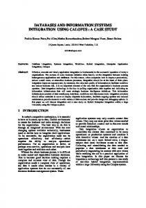
FINDING THE NEAREST OBJECT

zk24

• Ex: find the nearest object to P 12

8

7

9

1

C

E 13

4B5 2 A3

P

D 10

6

11 new F F

• Assume PR quadtree for points (i.e., at most one point per block) • Search neighbors of block 1 in counterclockwise order • Points are sorted with respect to the space they occupy which enables pruning the search space • Algorithm: 1. start at block 2 and compute distance to P from A 2. ignore block 3 whether or not it is empty as A is closer to P than any point in 3 3. examine block 4 as distance to SW corner is shorter than the distance from P to A; however, reject B as it is further from P than A 4. ignore blocks 6, 7, 8, 9, and 10 as the minimum distance to them from P is greater than the distance from P to A 5. examine block 11 as the distance from P to the southern border of 1 is shorter than the distance from P to A; however, reject F as it is further from P than A • If F was moved, a better order would have started with block 11, the southern neighbor of 1, as it is closest

9 8 7 6 5 4 3 2 1 v g z r v g z r b

PM1 QUADTREE

zk25

Vertex-based (one vertex per block)

a

b

h e

g

i

f

d c

DECOMPOSITION RULE: Partitioning occurs when a block contains more than one segment unless all the segments are incident at the same vertex which is also in the same block Shape independent of order of insertion

zk26 SAND BROWSER: A SPATIO-RELATIONAL BROWSER • Assume a relational database • Relations have spatial and nonspatial attributes • Browse through tuples or objects (groups of tuples with similar attribute values) of a relation one at a time according to values within ranges of the 1. nonspatial attributes 2. underlying space in which the objects corresponding to the spatial attributes are embedded • Make use of indexes to facilitate viewing (termed ranking) tuples in order of “nearness” to a reference attribute value (e.g., zero, origin, etc.) and obtain tuples in this order • Graphical user interface instead of SQL but functionally equivalent • Graphical result of spatial and nonspatial queries • Output 1. display tuples satisfying the query one tuple or one object at a time • show the values of all of the attributes of the most recently generated tuple • cursor points at this tuple 2. cumulative display of spatial attributes • Can save the result of an operation as a relation for future operations (SAVE GROUP)

zk27 SAND RELATION OR OBJECT DESCRIPTION • Assumes a relation 1. length: number of tuples 2. width: bytes per tuple • only accounts for fixed size components of a tuple • e.g., for a polygon, there is extra space needed for each vertex of the polygon • List of attributes 1. attribute names and type • e.g., name is a 25 character array • e.g., verts is a polygon 2. measurement type (e.g., nominal, ordinal, interval, ratio) • range of possible values for nominals if finite • range, if known, for interval and ratio 3. rendering attributes (e.g., color, iconic) 4. highlighting method 5. print name for tuple(s) or objects being displayed • Indexes 1. name of index 2. type of index • e.g., B-tree • spatial index and type 3. sort sequence • e.g., alphabetic • spatial a. sorted with respect to distance from Chicago b. no reference point (with respect to space occupied)

zk28 RENDERING ATTRIBUTES FOR SPATIAL RELATIONS: SPATIAL ATTRIBUTES 1. Set by user at query time or pre-defined at relation creation time 2. For entire relation or on a tuple-by-tuple basis 3. Examples: • line and fill colors, line thickness, point size • highlight method • what is being displayed a. boundary b. interior — need to fill when zoom in but can avoid fill if draw boundary after interior c. boundary plus interior 3. Name of type of objects being displayed • useful in dialog box for scan order so user knows what each tuple represents • e.g., Silver Spring map contains tuples corresponding to road segments 4. Scale for queries involving distance • used when zooming while specifying a query

zk29 VALUES OF RENDERING ATTRIBUTES FOR SPATIAL RELATIONS: SPATIAL ATTRIBUTES • Coloring choice method to automatically differentiate between displayed entities 1. specific color • e.g., blue meaning all are displayed in blue 2. different from previous • color is different from that of the tuple or object most recently displayed 3. different from adjacent • color is different from that of any spatially adjacent tuple or object • e.g., a side in common for regions and surfaces and a vertex for lines • Highlighting 1. shape • pre-defined such as rectangle, minimum bounding box, circle, etc. • user-defined graphically 2. color • fixed • arbitrary • different from colors of objects in the highlighted area 3. mode • blinking or non-blinking (i.e., binary)

zk30 RENDERING ATTRIBUTES FOR SPATIAL RELATIONS: NON-SPATIAL ATTRIBUTES 1. Scalar value or iconic rendering is displayed for each tuple • using the same rendering for different objects at different locations conveys a notion of similarity • e.g., company trademark to mark all its properties such as plants, stores, fields, ... • dissimilarity of rendering emphasizes differences between objects (e.g., different size circle for different cities based on their populations • may need a legend to convey the semantics of the different renderings 2. One attribute for the entire relation 3. Need to indicate position of displayed value • absolute location OR • relative to spatial attribute value 4. Icon for specifying the attribute value in a condition • e.g., slider for a ratio attribute • e.g., check box for a nominal attribute

zk31 SAND SPATIAL BROWSING CONSTRAINTS • Range 1. all tuples overlapping an object (spatial selection or a window query) • also termed a spatial join if a non-constant window 2. all tuples within a distance of an object (spatial range query) • also termed a spatial join 3. Boolean combinations of the above • Upper bound on the maximum number of tuples that can be found

zk32 SAND SPATIAL BROWSING ORDERINGS 1. Random order 2. In order of nearness to a particular object (termed a ranking object) • can limit the ordering to a range of distance values from the ranking object • ranking object need not be the same as the object a. being overlapped, OR b. in whose range we are retrieving • e.g., rank all streets within 10 miles of Georgia Ave. in the order of their distance from University Blvd. — a 3-way spatial join • could possibly be in order of farness (FUTURE!) 3. Could have multiple ranking objects with some priority • rank objects with respect to a polygon • rank objects with respect to a point • all objects within the polygon have a distance 0 and the tie is broken by ranking them with respect to the point 4. Cardinality or frequency • useful for finding which country has the most instances of a particular spatial feature • probably need to precede with a join • more useful for nonspatial attributes such as finding all cities with the same population and can use actual value of the attribute as a secondary ranking key

zk33 PRIMITIVE BROWSER SETTINGS 1. Scan Order: which attribute values form the basis of the browsing • assumes that an index exists for the attributes • can be a combination of attributes (e.g., name and type for street proper name and nature of street — i.e., “Avenue”) 2. Conditions: • Boolean combination of condition values of various attributes including ranges for attributes of type ratio and interval • take advantage of indexes on attributes, if they exist • future; graphical specification with icons from the rendering attributes 3. Display: output specifications 4. Browser Mode: • one tuple at a time (usual case!) even if several tuples have the same attribute value, OR • one object at a time a. retrieves all tuples with same attribute values b. condition specification is in terms of sets of attribute names • same spatial attribute value overcomes problem of spatial index resulting in more than one tuple per feature as in a disjoint decomposition such as a PM quadtree for lines • example a. retrieve all pieces of each segment of a polyline b. retrieve all pieces of a polyline

zk34 SAND BROWSER MENUS AND ACTION BUTTONS • File: browser control menu 1. Open: invoke SAND BROWSER on an additional relation • menu containing a schema for each relation (i.e., attribute names and types) • default values for rendering attributes on a relationby-relation basis 2. Save: make a relation from the tuples that satisfy the current browsing condition and save it • check box 3. Quit: exit SAND BROWSER • Display: output specifications menu • Options: anything else that was forgotten — a catch-all! 1. rendering attribute settings 2. name of type of objects being displayed (i.e., tuples) • Action buttons 1. First: first item in a particular scan order 2. Next: next item in a particular scan order • Mode radio button: 1. browse by tuples OR 2. browse by objects (sets of tuples) • Condition menus 1. spatial 2. non-spatial

zk35 SAND BROWSER SAVE MODES • Two modes: 1. FULL: tuples satisfying entire query • need to let query execute to completion if invoked in middle of ranking process • save entire relation if no ranking condition has been specified 2. PARTIAL: tuples computed so far • enables saving results of a partial ranking (e.g., nearest 5 neighbors) • Should also form indices for the attributes 1. copy existing indices • can be just a subset of the indices 2. new indices • Create a name for the objects represented by the relation’s tuples • Rendering attributes • Not a view as tuples are copied when forming new relation 1. difficult to implement views as they represent a sequence of operations that are applied to a database of relations • like common subexpression elimination for query expression • view is not precomputed 2. if any modifications to relations, then must update view 3. implementing views in SAND BROWSER would require saving geometric query objects and ranking objects which have been input by the user as well as the operations that were performed

zk36 ISSUES IN SPATIAL DATABASES 1. Representation • bounding boxes versus disjoint decomposition 2. How are spatial integrity constraints captured and assured? • edges of a polygon link to form a complete object • line segments do not intersect except at vertices • contour lines should not cross 3. Interaction with the relational model • spatial operations don’t fit into SQL a. buffer b. nearest to ... c. others ... • difficult to capture hierarchy of complex objects (e.g., nested definition) 4. Spatial input is visual • need a graphical query language

zk37 5. Spatial output is visual • unlike conventional databases, once operation is complete, want to browse entire output together rather than one tuple at-a-time • don’t want to wait for operation to complete before output a. partial visual output is preferable • e.g., incremental spatial join and nearest neighbor b. multiresolution output is attractive 6. Functionality • determining what people really want to do! 7. Performance • not enough to just measure the execution time of an operation • time to load a spatial index and build a spatiallyindexed output is important • sequence of spatial operations as in a spatial spreadsheet a. output of one operation serves as input to another • e.g., cascaded spatial join b. spatial join yields locations of objects and not just the object pairs

zk38 CHALLENGES: 1. Incorporation of geometry into database queries without user being aware of it! • find geometric analogs of conventional database operations (e.g., ranking semi-join yields discrete Voronoi diagram) • extension of browser concept to permit more general browsing units based on connectivity (e.g., shortest path), frequency, etc. 2. Spatial query optimization • different query execution plans • use spatial selectivity factors to choose between them 3. Graphical query specification instead of SQL 4. Incorporation of time-varying data • how to represent rates? 5. Incorporation of imagery 6. Develop spatial indices that support both locationbased (“what is at X”?) and feature-based queries (“where is Y”?) 7. Incorporate rendering attributes into database objects or relations • queries based on the rendering attributes • Ex: find all red regions • query by content (e.g., image databases) 8. GIS on the Web and distributed data and algorithms 9. Knowledge discovery 10. Interoperability

zk39 SELECTED REFERENCES (Also see http://www.cs.umd.edu/~hjs/pubs.html) 1. C. Esperança and H. Samet, An overview of the SAND spatial database system, to appear in Communications of the ACM, 1997. http://www.cs.umd.edu/~hjs/pubs/sandprog.ps.gz 2. G. Hjaltason and H. Samet, Ranking in Spatial Databases in Advances in Spatial Databases —4th Symposium, SSD’95, M. J. Egenhofer and J. R. Herring, Eds., Lecture Notes in Computer Science 951, Springer-Verlag, Berlin, 1995, 83-95. http://www.cs.umd.edu/~hjs/pubs/incnear.ps 3. H. Samet, Spatial Data Structures in Modern Database Systems: The Object Model, Interoperability, and Beyond, W. Kim, Ed., Addison-Wesley/ACM Press, 1995, 361-385. http://www.cs.umd.edu/~hjs/pubs/kim.ps 4. H. Samet, Applications of Spatial Data Structures: Computer Graphics, Image Processing, and GIS, Addison-Wesley, Reading, MA, 1990. ISBN 0-20150300-0. 5. H. Samet, The Design and Analysis of Spatial Data Structures, Addison-Wesley, Reading, MA, 1990. ISBN 0-201-50255-0. 6. H. Samet and W. G. Aref, Spatial Data Models and Query Processing in Modern Database Systems: The Object Model, Interoperability, and Beyond, W. Kim, Ed., Addison-Wesley/ACM Press, 1995, 338-360. http://www.cs.umd.edu/~hjs/pubs/kim2.ps 7. C. D. Tomlin, Geographic Information Systems and Cartographic Modeling, Prentice-Hall, Englewood Cliffs, NJ, 1990. ISBN 0-13-350927-3.