RIVER RESEARCH AND APPLICATIONS
River Res. Applic. 32: 1493–1504 (2016) Published online 18 December 2015 in Wiley Online Library (wileyonlinelibrary.com) DOI: 10.1002/rra.2990
SPATIAL DISTRIBUTION AND HABITAT USE OF SPAWNING AMERICAN SHAD IN THE ST. JOHNS RIVER, FLORIDA A. C. DUTTERERa*, W. E. PINE IIIb, S. J. MILLERc, A. R. HYLEd AND M. S. ALLENe a
Florida Fish and Wildlife Conservation Commission, Fish and Wildlife Research Institute, Gainesville, Florida USA b Wildlife Ecology and Conservation Department, University of Florida, Gainesville, Florida USA c St. Johns River Water Management District, Palatka, Florida USA d Florida Fish and Wildlife Conservation Commission, Fish and Wildlife Research Institute, Melbourne, Florida USA e Fisheries and Aquatic Sciences Program, University of Florida, Gainesville, Florida USA
ABSTRACT American shad Alosa sapidissima populations along the Atlantic Coast of North America are near historic lows despite management actions designed to rebuild stocks. Florida’s St. Johns River supports the southernmost population of this anadromous species, and as water use in the St. Johns basin increases, there is concern that their spawning may be affected. We assessed American Shad movement and habitat use in the St. Johns River during three spawning migrations (2009–2011) using acoustic telemetry. Spatial distribution patterns of telemetered shad during each year were largely similar; most shad were located within reaches from Lake Monroe (rkm 276) to just downstream of Lake Harney (rkm 308); some individuals made excursions as far upstream as Lake Poinsett (rkm 386+). Water levels varied among years (low-water level: 2009 and 2011; higher water level: 2010), and lower water levels may have contributed to an apparent constriction of spawning grounds in 2009 and 2011. Telemetered shad selected deeper sections of river with faster currents. Our results verified that the primary spawning grounds for American shad in the St. Johns have not changed substantially in the past 50 years; thus, these areas should rank high for habitat protection. We also demonstrated linkages between American Shad distribution and habitat use and river flow that should be further developed and considered in future water withdrawal, regulation, or conservation efforts. Copyright © 2015 John Wiley & Sons, Ltd. key words: Alosa sapidissima; anadromous fishes; spawning migrations; acoustic telemetry; river flows and levels; coastal rivers Received 06 May 2015; Revised 02 October 2015; Accepted 16 November 2015
INTRODUCTION Stream flow can strongly influence riverine fish communities by altering available habitat, water quality, food availability, spawning success, and predation risk (Cushman, 1985; Freeman et al., 2001; Murchie et al., 2008). Many riverine ecosystems in Florida, including the St. Johns River, are characterized by (1) low-elevation gradients that allow for large inland tidal and species incursions, (2) extensive connections between marine and freshwater fish and invertebrate communities, which create dynamic trophic and ecological interactions (Garman and Macko, 1998; Hall et al., 2012; Lauretta et al., 2013), and (3) widespread connections between surface and subsurface water due to karst and other porous geologic forms, which allow groundwater withdrawals to affect surface water levels (Belaineh et al., 2012). Changes to ecosystem structure and function in these systems will occur because of water withdrawals, which alter riverine flow and thus essential habitats and trophic
*Correspondence to: Andrew C. Dutterer, Florida Fish and Wildlife Research Institute, Florida Fish and Wildlife Conservation Commission, 7386 NW 71st St., Gainesville, Florida 32653, USA. E-mail:
[email protected]
Copyright © 2015 John Wiley & Sons, Ltd.
linkages. Many relationships between flow characteristics and ecosystem function, however, are poorly understood. Their elucidation through applied research is critical because river-flow and river-level regulations are being established across Florida to help water resource planners meet human water needs while minimizing impacts on natural resources. One species that is affected by river flows and levels is American Shad Alosa sapidissma, which is native to the East Coast of North America from the St. Lawrence River in Canada to the St. Johns River in Florida (Limburg et al., 2003). Abundance of anadromous shads (Alosa spp.) along the Atlantic Seaboard is at historic lows as a result of past high exploitation rates in riverine and oceanic habitats, widespread changes to riverine hydrology, and migratory barriers such as dams (Limburg and Waldman, 2009). Preserving anadromous shad stocks and rebuilding population status of these ecologically and culturally important species are an important goal for East Coast state and federal management agencies (ASMFC, 2010; McBride, 2014). Historically, anadromous shads supported important commercial and recreational fisheries in the St. Johns River during annual riverine spawning migrations. Commercial shad fishing started in Florida in 1858 and quickly gained momentum
1494
A. C. DUTTERER ET AL.
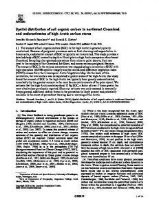
(Walburg, 1960). Around 1900, shad landings represented the highest value marine product for the state (McBride, 2000). For many years, Florida’s American Shad stock supported substantial commercial fishing, but landings began to decline in the 1960s, and commercial fishing was phased out (Figure 1). The Florida Limiting Marine Net Fishing Amendment ended in-river commercial fishing in 1995, and the ocean-intercept fishery for mixed stocks of shads in offshore waters ended in 2005 (ASMFC, 2010). Recreational fishing for this species, however, continues across its range; in Florida, the recreational harvest is regulated with a 10-fish daily bag limit (McBride and Holder, 2008). Conservation of anadromous fishes in Florida, including American Shad, is also furthered by statutes protecting their freshwater habitats. Regulations setting minimum flows and levels limit water use permitting to prevent ‘significant ecological harm’ to surface waters (Florida Statute 373), and protection of water levels needed to maintain fish passage is required by administrative code guidelines (Florida Administrative Code Chapter 40D-8, as an example). But despite regulation of shad fisheries and these basic habitat protection measures, Florida’s American Shad stock remains near its lowest levels (McBride, 2005; McBride and Holder, 2008). Mainstem dams are absent in the St. Johns, but river flows and levels have been altered by extensive hydrologic modification in the headwaters for agricultural and urban water supply and by extensive subsurface withdrawals throughout the basin (NRC, 2009). The cumulative, long-term ecological effects of these hydrological changes are unknown and could contribute to delayed recovery of shad in the St. Johns. Hydrologic conditions affect habitat use, movement, growth, and survival of anadromous shads during juvenile and adult freshwater residency. A review of the potential impacts of low river flows on American shad in the St. Johns (Harris and McBride, 2004) expressed concern that in-river spawning migration and habitats of adult shad and downstream emigration of juveniles could be affected by river flows. They reviewed known spawning habitats and egg and larval requirements for shad in the St. Johns and elsewhere, and concluded that when
eggs and larvae are developing in the St. Johns (December– May), maintaining appropriate flow rates is important. However, much of the material reviewed by Harris and McBride (2004) has become dated, and much of what is known about American Shad spawning in the St. Johns was provided by the work of William and Bruger (Williams and Bruger, 1972), which occurred over 40 years ago. Given increasing demands by humans for water resources in the St. Johns basin, an updated view of where American Shad spawn and of how river flow influences the spatial distribution of spawning adults would be valuable. Our objectives were to assess the spatial distribution and habitat selection of American Shad during spawning migrations in the St. Johns by monitoring movements and habitat use of telemetered fish through a fixed acoustic receiver array supplemented with mobile tracking. We then compared these results with sampling data from the 1960s to assess whether spawning areas have shifted as human development and water use patterns have changed. METHODS Study site The St. Johns is the largest river located entirely within Florida and is hydrologically unusual in several respects. Its headwaters are found in southern Florida near Melbourne, from which it flows north paralleling the Atlantic coast through an intermittent series of natural lakes to its mouth in north Florida, near Jacksonville (Belleville, 2000). Along this distance of approximately 500 km, river elevation changes only 8 m (McBride and Holder, 2008), resulting in slow currents and extensive tidal influence (200–270 km upstream). Although the St. Johns has no mainstem dams, it supplies critical water resources to many agricultural, industrial, and municipal users. The hydrology of the upper basin was altered for agricultural use (e.g. diking and draining of marshes with construction of canals) and flood control (e.g. water diversion canals) during the early to mid-1900s, but large restoration projects have been ongoing since the 1970s (SJRWMD, 2007). Previous research on American Shad spawning in the St. Johns indicated that discharge and water level likely influenced the distribution of spawning fish (Williams and Bruger, 1972), so knowledge of water levels during our research provides important context to the spatial distribution patterns of our telemetered shad. We selected a US Geological Survey gauge 02234000 on the St. Johns at rkm 316 (Figure 2) to classify water level because it was central to the historic shad spawning grounds (Williams and Bruger, 1972). Tagging
Figure 1. Landings (metric tons) of American Shad for Florida and
the US Atlantic Coast, 1950–2012 (NOAA, 2014) Copyright © 2015 John Wiley & Sons, Ltd.
We used acoustic telemetry to track adult shad during their freshwater migration to verify spawning grounds and measure River Res. Applic. 32: 1493–1504 (2016) DOI: 10.1002/rra
1495
AMERICAN SHAD SPAWNING AT ST. JOHNS RIVER
Figure 2. Discharge (top) and stage (bottom) during the American Shad spawning season (December–May) at US Geological Survey gauge 02234000 on St. Johns River for 3 years of this study (2009–2011), 2 years of the Williams and Bruger (1972) study (1969 and 1970) and median gauge values (discharge: 1981–2011; stage: 1941–2011)
habitat characteristics. We assumed that overall distribution of telemetered shad reflected the spawning grounds, and that specific locations of individuals reflected habitat important for spawning. American Shad are fractional spawners, releasing eggs every 2–3 days, and so remain in or near suitable spawning habitat while on the spawning grounds (Hyle et al., 2014; Hyle AR, unpublished research). We collected shad for tagging during January and February (2009–2011). Historically, the earliest American Shad entered the St. Johns in late November or December. Shad abundance and spawning activity typically increased to a peak in February and March and subsided by May (Williams and Bruger, 1972; Davis, 1980; McBride and Holder, 2008). Our sampling was intended to collect shad as early as possible and as they approached the downstream reaches of the spawning grounds. During each spawning season, we staggered the release of tagged fish over multiple sampling events to disburse transmitters among different entrant groups. We collected adult shad via boat electrofishing (Smith-Root Inc. 9-kW generator powered pulsator) and selected individuals ≥400 mm total length (TL) for tagging. Based on our analysis of historical shad length and weight data collected by Florida Fish and Wildlife Conservation Commission during 2002–2007 (n = 3129) and reported by McBride and Holder (2008), over 95% of American Shad sampled in the St. Johns in January and February that were ≥400 mm TL were also ≥530 g. Thus, the Copyright © 2015 John Wiley & Sons, Ltd.
tag-weight:body-weight ratio was likely ≤2% for most of our tagged shad (Winter, 1996). We tried to collect and tag shad before they reached spawning areas. But because much of the St. Johns downstream of the historic shad spawning grounds is deep (>2.5 m) and wide (>3 km), with high conductivity (primarily from groundwater sources upstream of rkm 100; Belaineh et al., 2012), capture efficiency of shad with our boat electrofishing gear in these areas was too low to produce needed sample sizes. Thus, we had to target reaches immediately downstream of historic spawning reaches. In 2009, shad were tagged between rkm 279.5 to 280.5 (a small section of channels between Lake Monroe and S.R. 415), and during 2010 and 2011, we tagged most fish between rkm 266.6 and 267.4. However, in 2010, we tagged five shad in the lower river, between Palatka (rkm 133) and Lake Dexter (rkm 215). We used Vemco V-13 ultrasonic transmitters (13-mm diameter × 36 mm long; 10.6 g; 101-d projected tag life; 69.0 kHz) and implanted them using a nonsurgical, esophageal-implant method common in shad telemetry studies (Bowman, 2001; Olney et al., 2006; Harris and Hightower, 2011). For implantation, we coated transmitters with water-soluble surgical lubricant and held them in the end of a thin-walled acrylic tube (13.5 mm inside diameter; 15.8 mm outside diameter). Via the tube, we pushed the transmitter through the oesophagus into the stomach where it remained during the spawning migration. To minimize handling stress, we minimized captive time. We tagged each shad within 2–3 min of capture. After tag insertion, we monitored shad in a holding tank of aerated river water for approximately 30 s for any signs of tag regurgitation (which was not observed for any individuals) and to verify that they had recovered from the sedative effects of electric shock. We returned shad to the river as soon as self-maintained equilibrium and steady swimming speed were verified. Fixed-position receiver array We monitored movement of tagged shad via an array of fixedposition Vemco VR2 or VR2W omni-directional hydrophones and acoustic receivers (Figure 3). Based on range testing, our receivers covered a detection radius of 200–300 m. We stationed acoustic receivers in channel constrictions, where the width of the river was less than that detection radius to maximize the chance of detecting passing tagged shad. During the 2009 spawning season, most positions within the acoustic receiver array had two receivers, offset by up to 100 m, but monitoring the same locality. Detection patterns were the same for all paired receivers in 2009, and manual tracking revealed no detection gaps, which we interpreted as evidence for high (near 1) detection probability for each receiver in the array. Receivers identified each tagged fish as it passed and recorded River Res. Applic. 32: 1493–1504 (2016) DOI: 10.1002/rra
1496
A. C. DUTTERER ET AL.
Figure 3. Map of the St. Johns River showing the proportion of individuals from each annual cohort of tagged American Shad detected at each stationary hydrophone receiver (circles) that served as check stations along the river. Cross symbols represent zero detection; open circles are scaled to show proportional values
date and time. Positioning of receivers was designed to monitor movements of shad over much of the upstream reaches of the St. Johns while focusing on reaches previously identified as supporting spawning (Williams and Bruger, 1972). We stationed one or two receivers downstream of locations where shad were collected so that we could identify instances of a tagged shad’s abandoning the spawning migration. We also stationed receivers in the Econlockhatchee River, a tributary of the St. Johns that supports shad spawning (Williams and Bruger, 1972). In all years, we had one receiver ~300 m inside the mouth of the Econlockhatchee; but in 2010 and 2011, we stationed a second receiver approximately ~18 rkm upstream of the Econlockhatchee-St. Johns confluence (Figure 3). Each acoustic transmitter emitted an identifying signal at a semi-random interval, ranging from 15 to 45 s (mean = 30 s). This transmission frequency, coupled with approximate swimming speed (approximately 1 body length/s), increased the likelihood that migrating fish would not travel through a monitoring gate undetected. To assess upstream migrations of our tagged shad, we plotted the fraction of tags at large that were detected at each receiver over the entire season. This allowed us to evaluate what fraction of our tagged shad made lengthy migrations upstream through the receiver array. To understand which reaches were most heavily used through time, we weighted individual fish detections on a daily time scale. For each receiver, we tallied the number of unique tagged shad recorded per day (referred to as fish · day 1). With Copyright © 2015 John Wiley & Sons, Ltd.
this format, detection of a fish that briefly passed a receiver was the same as continually recording a fish at a single receiver over an entire day—both scenarios equaled one count in the fish · day 1 tally. When plotted across the entire spawning season, cumulative fish · day 1 at each receiver allowed us to distinguish reaches that were consistently occupied by tagged shad for multiple days or weeks from reaches where shad had only passed through. This did not preclude a fish’s being detected on multiple receivers on the same day. Manual tracking During the 2010 and 2011 spawning seasons, we conducted manual telemetry searches (Vemco VR-100 receiver and directional hydrophone) for tagged shad to complement the fixed-position receiver array. Our searches were stepwise, the search boat advancing incrementally along a river reach based on tag detection range; the directional hydrophone was used, while the search boat was relatively stationary. One stepwise, incremental searching effort along a river reach was referred to as a pass, and these were conducted approximately biweekly while transmitters were viable. Our manual searches covered an average of 17 rkm per day. When a tagged shad was located via manual tracking, we evaluated signal strength from multiple locations to triangulate, as precisely as possible, the individual’s location. Our margin of error for triangulation varied with environmental River Res. Applic. 32: 1493–1504 (2016) DOI: 10.1002/rra
1497
AMERICAN SHAD SPAWNING AT ST. JOHNS RIVER
conditions. Based on range testing, triangulation was accurate to within 1–2 m under optimal conditions, but under adverse conditions, accuracy was reduced to tens of metres because transmitter signal strength was difficult to differentiate for triangulation at close range, when there was high ambient noise, or if a telemetered fish moved in response to the presence of the tracking boat. Nonetheless, once the best position fix could be obtained, we recorded latitude and longitude with a GPS and measured habitat parameters (detailed later). Habitat assessment We recorded depth (m; using a measuring staff or a sonar unit), current velocity (m ∙ s 1; using a Marsh-McBirney Flo-Mate 2000 digital flow meter), and substrate type at the river channel thalweg closest to each manually relocated shad. Substrate was sampled via a steel pipe dredge (102-mm diameter, 406-mm length and 4.54 kg) lowered to the substrate and dragged for approximately 1 m. Substrate type was classified visually into one of five categories based on predominant composition (sand, sand > silt, sand = silt, silt > sand or silt; Dutterer et al., 2011). Initial manual searches indicated that telemetered fish were usually located in the thalweg, and we used the thalweg as a proxy for shad location if triangulation was not possible. To determine whether spawning shad selected for certain habitat conditions in the St. Johns (i.e. whether habitat use differed from random locations), we compared habitat parameters for areas where telemetered shad occurred with those measured at random locations that represented available habitat. Randomized points along the river centerline were generated prior to the spawning season. At the beginning of each day of manual searching, a subset of these coordinates within the day’s sampling reach were randomly selected (without replacement) for available habitat measurements. Thus, we continuously measured available habitat conditions throughout the spawning season, and these measurements reflected any changes in water levels during the spawning season. We tested for differences between used and available depth and current velocity with two sample t-tests and substrate categories with a chi-squared test. We considered that habitat selection had occurred if there was a significant difference (α = 0.05) between used and available measures (Rosenfeld, 2003; Dutterer and Allen, 2008). Comparison to previous American Shad spawning Williams and Bruger (1972) mapped the spatial distribution of spawning American Shad in the St. Johns in 1969 and 1970 by collecting shad eggs via fixed-position plankton nets. Although our studies collected different information for inference of spawning locations (egg locations vs. adult locations), the data from the two studies could be compared spatially by standardizing per unit of sampling effort (eggs ∙ hr 1; telemetered shad detected ∙ pass 1). We calculated catch per unit effort (CPUE) Copyright © 2015 John Wiley & Sons, Ltd.
for each rkm that was searched at least once via manual telemetry; CPUE was measured as the total number of telemetry tag detections divided by number of searching passes completed with manual telemetry gear. We obtained average egg catch ∙ hr 1 data from William and Bruger (Williams and Bruger, 1972; Tables 1 and 4 within), who mapped sampling locations and river mile landmarks (see Figure 3 in Williams and Bruger, 1972). To standardize spatial values between the two studies, we assigned rkm values to Williams and Bruger’s (1972) catch data based on comparison of their map with one we generated in a geographic information system ArcGIS. This allowed direct graphical comparison of Williams and Bruger’s (1972) egg catch records with our telemetry relocation data.
RESULTS Water levels River discharge and water level varied among years of our study, resulting in one high-water-level year (2010) and two low-water-level years (2009 and 2011; Figure 2). These classifications were based on water levels during the shad spawning season (December–May) relative to median water levels for gauge history (stage: 1941–2012; discharge: 1981–2012). Compared with those for sampling in 1969 and 1970 by Williams and Bruger (1972), water levels were higher from December through March in 1970 than in any of the three years of our assessment. River levels were higher from mid-March through June during our high-water year of 2010 than in 1969 or 1970. Shad collection and tagging Through 3 years of spawning migrations, we tagged 114 American Shad with acoustic telemetry transmitters. All tagged shad were 400 mm TL or longer (range: 400–526 mm TL), and we tagged a similar number of males and females. All tagging occurred in January and February, and the number of tagging events per season ranged from 3 to 7 (Table I). Fixed-position receiver array Movement patterns within the fixed-position receiver array were similar from year to year over three spawning seasons of monitoring. In each year, the greatest number of telemetered shad occurred between lakes Monroe and Jesup (rkm 276–287; Figures 3 and 4), and detections of shad steadily declined upstream from that reach. During 2009–2011, 80%, 52% and 53% of the telemetered shad during each year, respectively, did not ascend beyond Lake Harney (rkm 308). Detection histories from the fixedposition receiver array showed that 7–18% of tagged shad entered the Econlockhatchee River during each year of our study (Figure 3) and were observed to migrate as far as River Res. Applic. 32: 1493–1504 (2016) DOI: 10.1002/rra
1498
A. C. DUTTERER ET AL.
Table I. Number of telemetry tags, TL range, number by sex, tagging date range, and total tagging events, by year of study Sex Year
Telemetry tags
TL (mm) range
M
F
Tagging date range
Total tagging events
2009 2010 2011
15 59 40
400–483 404–490 401–526
— 29 17
— 30 23
26 Jan–12 Feb 18 Jan–22 Feb 12 Jan–10 Feb
3 7 5
TL, total length.
18 rkm upstream. We observed that, post tagging, 6–10% of shad in all years delayed or abandoned typical upstream spawning migration (which Olney et al. [2006] called fallback), but most shad exhibiting fall-back eventually resumed upstream movement and reached the spawning grounds. Although overall detection patterns among years shared several similar patterns, the number of shad that migrated to the upstream extents of the fixed-position receiver array varied somewhat among years (Figures 3 and 4). In 2009 and 2011, the lower-streamflow years, tagged shad were detected only as far upstream as rkm 350.5–362.1. During 2010, the high-streamflow year, we detected 12 shad (24%) at rkm 350.5 and 5 (10%) that ascended to the last upstream monitoring station at rkm 386.6. Thus, the distance travelled upstream by spawning shad increased with greater water levels among years.
Manual tracking Tag detection patterns via manual telemetry were similar in 2010 and 2011 (Figure 5) and showed similar spatial distribution patterns for shad as documented by the fixed-position receiver array each year. Searching efforts were similar between years as we searched 690 and 737 cumulative rkm in 2010 and 2011, respectively. During both years, we were able to relocate a large proportion of our tagged fish via manual searches, detecting 53 of 59 in 2010 and 34 of 40 in 2011. Telemetry CPUE varied from 0 to 2.63 detections ∙ pass 1 in 2010 and from 0 to 2.11 detections ∙ pass 1 in 2011. In both years, the highest telemetry CPUE for shad occurred in the reach between lakes Monroe and Jesup (rkm 279–283). In 2010, we observed secondary peaks in telemetry CPUE at rkms 313, 326 and 357 (1–1.33 detections ∙ pass 1). In 2011, we observed secondary peaks in telemetry CPUE at rkms
Figure 4. Map of the St. Johns River showing the proportion of cumulative fish ∙ day
1 logged at each stationary hydrophone receiver (circles) that served as check stations along the river. Cross symbols represent zero detection; open circles are scaled to show proportional values
Copyright © 2015 John Wiley & Sons, Ltd.
River Res. Applic. 32: 1493–1504 (2016) DOI: 10.1002/rra
AMERICAN SHAD SPAWNING AT ST. JOHNS RIVER
1499
Figure 6. Frequency distributions of depths at river thalweg where
manually telemetered American Shad were located (used habitat; black bars) and randomly selected thalweg depths (available habitat; grey bars)
Figure 5. Plots of American Shad egg catch per unit effort [catch per unit effort (CPUE); eggs ∙ hr 1] during 1969 and 1979 and telemetry CPUE (tag detections ∙ pass 1) in 2010 and 2011. Plots of shad egg CPUE were created from Tables 1 and 4 and Figure 3 in Williams and Bruger (1972)
326 and 341 (0.8–1.0 detections ∙ pass 1). Differences in telemetry CPUE between years occurred primarily in the most upstream range of shad movements, with detections of shad extending much farther upstream in 2010 (high-water levels) than in 2011 (low-water levels). Thus, our manual telemetry results showed the same distribution of spawning shad that was documented via the stationary receiver array.
of telemetered shad (Figure 7). Thus, mean current velocity at channel thalweg for habitats used by shad (0.119 m ∙ s 1; n = 128) was significantly greater (d.f. = 204, p = 0.0032) than mean current velocity at random locations (0.092 m ∙ s 1; n = 78), indicating that American Shad selected for deeper sections of river with higher current velocities. In contrast to depth and velocity, evidence for substrate selection was less apparent. A chi-square test indicated that telemetered shad did not use our substrate categories at the same frequency as the categories occurred in our randomized substrate samples (X2 = 15.676; d.f. = 4; p = 0.0035). However, differences between used and available substrate categories did not show a pattern along the gradient of particle size (i.e. from larger sand particles to smaller silt particles; Figure 8). A literal interpretation of the chi-square test result and frequency distribution of substrate categories would suggest that our telemetered shad selected for areas of pure silt and substrates in which sand was dominant over silt,
Habitat selection We located tagged shad in habitats where the maximum depth ranged from 0.5 to 7 m and thalweg current velocity ranged from 0.01 to 0.31 m ∙ s 1. The frequency distributions of depths for used and available habitats showed similar range, but there was greater incidence of deeper depths corresponding to locations of telemetered shad (Figure 6). Thus, mean depth at channel thalwegs used by shad (2.73 m; n = 130) was significantly deeper (d.f. = 205, p = 0.0045) than thalweg depths at our randomized locations (characterizing available habitat conditions; mean = 2.24 m; n = 77). Likewise, the frequency distributions of current velocity measures for used and available habitats showed similar range, but there was greater incidence of faster flows corresponding to locations Copyright © 2015 John Wiley & Sons, Ltd.
Figure 7. Frequency distributions of current velocities at river
thalwegs where manually telemetered American Shad were located (used habitat; black bars) and randomly selected thalweg current velocity (available habitat; grey bars) River Res. Applic. 32: 1493–1504 (2016) DOI: 10.1002/rra
1500
A. C. DUTTERER ET AL.
studies suggest that most American Shad spawning in the St. Johns has occurred within the same ~100 km of river channel each year, but locations of peak spawning activity can vary substantially between years or sampling technique.
DISCUSSION
Figure 8. Frequency distributions of substrate categorizations corresponding to areas used by telemetered American Shad (black bars) and randomized locations that characterized available conditions (grey bars)
while avoiding substrates of pure sand, areas of equal parts sand and silt and areas where silt was dominant over sand. However, a literal interpretation of these results made little biological sense and, in our opinion, was overshadowed by no clear pattern of selection along the gradient of particle sizes in the frequency distribution of substrate categories (Figure 8). Thus, our interpretation of these results was that they do not present compelling evidence for substrate selection among our telemetered shad. Comparison with historical spawning information The reaches used by our tagged shad fell within the same overall range of historical egg collections in the St. Johns, but the relative importance of smaller reaches within the overall spawning grounds varied somewhat among studies. Williams and Bruger (1972) commonly collected eggs between rkms 275 and 390, and that section of the river is where almost all of our telemetered fish were found during each spawning season of our study. Peak detections for shad in our study were consistently centred between lakes Monroe and Jesup, near rkm 280. This reach produced large catches of American Shad eggs in 1953 for Walburg (1960) and in 1970 for Williams and Bruger (1972). But Williams and Bruger (1972) consistently observed their largest egg catches 50–100 rkm upstream of our high-use reach (Figure 5). Nichols (1965, 1966) also monitored American Shad spawning on the St. Johns by collecting eggs and reported highest catch rates in 1964 between rkm 350.5 and 386.6 and near rkm 330 (also, 50–100 rkm upstream of our high-use reach) for 1965. McBride and Holder (2008) reported electrofishing catches of American Shad during 2002–2005, and in contrast to our results, their catches from reaches near lakes Puzzle and Cone and the Econlockhatchee River (all upstream of rkm 314) were about threefold greater than those from reaches between lakes Monroe and Harney. The combined results of these Copyright © 2015 John Wiley & Sons, Ltd.
This study represents the first assessment of the American Shad spawning grounds in the St. Johns based on telemetry of adults, and it provides the first broad-scale assessment of the American Shad spawning grounds there since the work of William and Bruger (1972), over 40 years ago. We documented locations and habitat use of adult American Shad during their spawning migration in the St. Johns River by tagging shad after they entered the river in winter and early spring and followed them to multiple river reaches upstream of Lake Monroe, where spawning likely occurred. Our observations were supported by independent identification of suitable spawning habitat (based on depth and current velocity surveys) for American Shad in these same reaches (Miller et al., 2012). Further, collections of juvenile or larval shad in this vicinity, or downstream of it, documented successful American Shad spawning in the St. Johns concurrent with each year of our study (Boucher, 2009; Holder et al., 2010, 2011). Overall, the spatial extent of American Shad spawning grounds in the St. Johns was basically the same as those documented 40 years earlier, which suggests that despite extensive hydrologic and landcover changes within the basin in this time period (SJRWMD, 2007), this series of river reaches continues to provide the primary suitable spawning grounds. Within this larger zone of historic shad use, our telemetered shad largely focused spawning activity (across all 3 years of study) in the relatively short reach between lakes Monroe and Jesup (rkm 275–287). We found that this apparent focal area was used for spawning during both high-river and low-river-discharge years, but we saw differences in upstream migration distances between the high-flow year and the two lower-flow years, with some shad making longer migrations during conditions of greater discharge. Our results suggest that the upstream migration distance of American Shad may have been influenced by water levels and flows. During our higher-water year of 2010, we detected 10% (n = 5) of the telemetered shad migrating to at least rkm 386.6, and we tracked three of these fish as far upstream as rkm 402.8. We did not detect any tagged fish migrating that far upstream during our low-water years of 2009 or 2011 (maximum upstream detections, rkm 350.5 and 362.1, respectively). Other studies corroborate these telemetry findings. During annual adult American Shad riverine sampling, shad were collected from these upper reaches (rkm 356–358) during very low water in 2007 and 2011 via airboat electrofishing, but catches farther upstream of a shallow sandbar at River Res. Applic. 32: 1493–1504 (2016) DOI: 10.1002/rra
AMERICAN SHAD SPAWNING AT ST. JOHNS RIVER
rkm 365 were very low (Holder et al., 2011; Hyle AR, unpublished research). High water conditions in 1970 (similar to our 2010 water levels) coincided with documented American Shad spawning well upstream at rkms 400 (near Lake Poinsett), 422 and 433 (Williams and Bruger, 1972). Thus, several lines of inference indicate that water level may affect the size of the spawning grounds. We observed telemetered shad in water with current velocities of 0.01–0.31 m ∙ s 1 (average: 0.12 m ∙ s 1), which was low compared with other reports. In most other systems in the southern portion of the American Shad range, shad spawn in currents several times faster than we observed (Massman, 1952; Facey and Van Den Avyle, 1986; Bowman, 2001; Hightower and Sparks, 2003). Interestingly, most of the shad eggs collected in the St. Johns by Williams and Bruger (1972) were also from reaches with faster current (0.3–0.46 m ∙ s 1). River stage, tide and wind patterns can contribute to variability in current velocity in the St. Johns, but low current velocities are characteristic, given its low gradient. Because of the overall slow flows of the St. Johns, it was not surprising that we observed selection for habitats with faster currents among our telemetered shad. Similarly, Bowman (2001) showed selection for faster than average currents by American Shad in the Neuse River, North Carolina. Several other studies have also linked shad spawning behaviours and habitat use with spatial distribution and variation in river flows, indicating that they select and require certain flows (often the fastest available currents). Leggett (1976) surmised that American Shad relied on steady downstream flows as cues for finding spawning habitat. When downstream flow stopped or reversed (as influenced by tides), he observed that shad stopped upstream movement or even moved downstream. Shad in the Santee River, South Carolina, shifted spawning migration routes toward a specific lock and dam as its discharge was markedly increased (Cooke and Leach, 2003). In 2004, Harris and McBride showed for the St. Johns that catch rates of American Shad eggs were significantly and positively correlated with current velocity. To explain the species’ apparent need for areas of increased river flow, Walburg and Nichols (1967) suggested that shad select these habitats to prevent their eggs from becoming trapped in silt and suffocating. Given the characteristic slow currents of the St. Johns, finding suitable current velocities for spawning may be especially important for shad, and possibly, this population experiences greater risk of diminished spawning success under altered hydrology or drought. We observed low diversity of substrate in the St. Johns, and we did not observe compelling evidence for substrates selection among telemetered shad. Williams and Bruger (1972) reported that catch of American Shad eggs in the St. Johns occurred over clean sand substrates, which differs somewhat from our results. They did not provide details for habitat categorization, and differences in our methods or Copyright © 2015 John Wiley & Sons, Ltd.
1501
subjectivity in substrate categorizations may explain the difference. Also, small-scale diel position adjustments (discussed later) or low resolution in triangulating fish position could have obscured substrate selection for spawning. Research on other river systems in which American Shad spawn has indicated that shad spawn over relatively coarse substrates, such as gravel, cobble or boulders (Stier and Crance, 1985; Bowman, 2001; Hightower and Sparks, 2003; Hightower et al., 2012). These substrates are typical of geomorphologic transitions between upland and coastal plain habitats, but they are not found in the St. Johns. We also found that shad selected for deeper habitats in our spawning reaches. American Shad spawning has been reported at a range of depths (Massmann, 1952; Stier and Crance, 1985; Bowman, 2001; Hightower and Sparks, 2003; Hightower et al., 2012). The wide range of substrate and depths used for spawning throughout the species’ range suggests that depth and substrate selection could be secondary to locating suitable current velocity. An underlying (and explicit) assumption of this project was that our telemetered shad were representative of overall behaviour and movement patterns of the American Shad spawning migration in each year. A potential criticism of this project is that by tagging shad, we affected their behaviour. We minimized the tag-weight:body-weight ratio (Winter, 1996) and handling time of tagged shad to minimize taginduced stress and saw no evidence to suggest that bearing a tag affected their behaviour, nor was this a major concern for multiple other American Shad telemetry studies that used the same tagging method (Bowman, 2001; Olney et al., 2006; Harris and Hightower, 2011). Nonetheless, it would have been difficult to discern if our tags elicited subtle changes in behaviour. Another potential criticism of our methods was that our timing or location for collecting and tagging shad could have biased results. Our high use reaches between lakes Monroe and Jesup began ~10 rkm upstream from where most of our shad were tagged. This could be viewed as low dispersion from the tagging site (reflecting a bias). Some shad were tagged in mid-February, near the peak of historic spawning activity, and those particular fish may not have had time to disperse to upper reaches of the river prior to spawning. However, 47% of our shad were tagged in January, and by the first week of February in each year, 80% of our shad were tagged. Thus, most of our shad were likely tagged prior to peak spawning activity and should have had time for continued migration well beyond the Monroe-Jesup, high-use reaches. Further, we saw no major differences in dispersion between early-tagged and late-tagged shad. In 2010, we were able to tag five shad between rkms 133 and 215 (51–133 rkm downstream from the primary tagging site). Albeit a small sample size, those individuals showed no notable differences in their migration patterns or habitat use relative to the other telemetered shad (i.e. they also exhibited high use of the reaches River Res. Applic. 32: 1493–1504 (2016) DOI: 10.1002/rra
1502
A. C. DUTTERER ET AL.
between lakes Monroe and Jesup) and helped to alleviate concerns of bias due to tagging location. Ours was the first study to use telemetry to follow adult American Shad during the spawning migration in the St. Johns, and differences between our findings and those of earlier studies could be due to differences in methodologies and gear biases used for assessing shad spawning (Harris and Hightower, 2010). Many studies relied on the collection of recently spawned eggs (Walburg, 1960; Nichols, 1965, 1966; Williams and Bruger, 1972). Because American Shad eggs are demersal, it has usually been assumed that they have been collected near spawning sites (Walburg, 1960; Williams and Bruger, 1972; Hightower and Sparks, 2003). But taking into account egg age, Harris and Hightower (2011) estimated that American Shad eggs in the Pee Dee River in North and South Carolina had travelled on average 24 rkm before collection, blurring somewhat the spatial precision of earlier studies addressing spawning locations of shad based on egg collection without staging (Harris and Hightower, 2010). Earlier research has indicated that American Shad usually spawn at night (Facey and Van Den Avyle, 1986; Bowman, 2001), but our manual telemetry searches (on which measures of used habitat relied) were conducted during the day. Thus, our tagged shad could have made short movements from their telemetered locations during the day to locations where spawning occurred (possibly at night). Harris and Hightower (2011) suggested that American Shad selected spawning reaches based on macrohabitat characteristics, likely making only small-scale position adjustments, if any, within these areas to spawn in optimal current or depth. Results from our fixed-position receiver array provided constant monitoring at a large spatial scale and did not indicate any large shifts in shad position between day and night, so any diel position shifts would have been small. Electrofishing catch of American Shad by McBride and Holder (2008) showed high relative catch rates among upstream reaches, such as near lakes Puzzle and Cone and within the Econlockhatchee River, contrasting our observation of highest use in the reaches between lakes Monroe and Jesup, which were much farther downstream. Generally, portions of the river upstream of Lake Harney have shallower and narrower channels, which would lead to higher efficiency with boat electrofishing gear (Bayley and Austen, 2002). Thus, some of the differences between high use areas in our study and McBride and Holder (2008) could be explained by differing gear efficiency along large-scale habitat gradients in the river. Based on our observations, reductions in river discharge and water level in the St. Johns from increased water withdrawals or changing climate could affect the success of American Shad spawning and rebuilding of the population by restricting access to spawning reaches or reducing the availability of habitat with the flow velocities suitable for spawning. Although we emphasize that reduced water levels Copyright © 2015 John Wiley & Sons, Ltd.
could have negative effects for shad, our study was not designed to make recommendations as to what level of hydrological modification or water withdrawal would be acceptable and still provide for adequate shad reproduction. Rather, we have verified that the species’ spawning grounds in the St. Johns remain focused on the same river reaches as documented decades ago. We also demonstrated additional support for linkages between shad spawning habitat and water levels proposed by numerous researchers (Walburg, 1960; William and Bruger, 1972; Harris and McBride, 2004). Therefore, water use and regulation in the St. Johns should take a cautionary approach regarding their effects on American Shad spawning habitat. This sentiment was voiced over 40 years ago by William and Bruger (1972), and their research helped to preserve the condition of much of the shad spawning grounds since then. Research and conservation efforts should continue to focus on the spawning grounds delineated in this and other investigations and continue to examine the effects of water level variation on American Shad reproduction. Future research should investigate population-level impacts of variable discharge and water level conditions on American Shad spawning success by relating annual water levels experienced by eggs and juveniles with age-specific abundance of adult cohorts when they return to the St. Johns to spawn. If water levels in the St. Johns do govern year-class strength, knowledge of this relationship could provide specific, quantitative guidance to water use and regulation within the basin. ACKNOWLEDGEMENTS
This work represents the collaboration of the Florida Fish and Wildlife Conservation Commission, the St. Johns River Water Management District and the University of Florida and was supported by Federal Aid in Sport Fish Restoration Program funds. Jay Holder, Dick Krause and Jim Estes provided considerable guidance in project development, implementation and interpretation. Ken Snyder, Kevin Johnson and Bob Eisenhauer provided airboat support and expertise in navigating the St. Johns. Darren Pecora, Zack Martin, Nick Cole and Zak Slagle provided extensive technical field assistance. Krystan Wilkinson and Mike Dodrill provided outstanding graphical and GIS support. Wes Porak, Bland Crowder and two anonymous reviewers contributed insightful editorial review.
REFERENCES ASMFC (Atlantic State Marine Fisheries Commission). 2010. Amendment 3 to the Interstate Fishery Management Plan for Shad and River Herring (American Shad Management). ASMFC: Washington. Bayley PB, Austen DJ. 2002. Capture efficiency of a boat electrofisher. Transactions of the American Fisheries Society 131: 435–451. Belaineh G, Stewart J, Sucsy P, Motz LH, Park K, Rouhani S, Cullman M. 2012. Groundwater hydrology. In St. Johns River Water Supply Impact River Res. Applic. 32: 1493–1504 (2016) DOI: 10.1002/rra
AMERICAN SHAD SPAWNING AT ST. JOHNS RIVER
Study, Lowe EF, Battoe LE, Wilkening H, Cullum M, Bartol T (eds). St. Johns River Water Management District, Technical Publication SJ20121, Palatka, Florida. Belleville B. 2000. River of Lakes: A Journey on Florida’s St. Johns River. University of Georgia Press: Athens. Boucher JM. 2009. Spawning Patterns and Larval Growth and Mortality of American Shad, Alosa sapidissima, in the St. Johns River, FL. Master’s thesis. Florida Institute of Technology: Melbourne. Bowman SW. 2001. American Shad and Striped Bass Spawning Migration and Habitat Selection in the Neuse River, North Carolina. Master’s thesis. North Carolina State University: Raleigh. Cooke DW, Leach SD. 2003. Beneficial effects of increased river flow and upstream fish passage on anadromous Alosine stocks. In Biodiversity, Status, and Conservation of the World’s Shads, Limburg KE, Waldman JR (eds). American Fisheries Society, Symposium 35: Bethesda, Maryland; 331–338. Cushman RM. 1985. Review of ecological effects of rapidly varying flows downstream from hydroelectric facilities. North American Journal of Fisheries Management 5: 330–339. Davis SM. 1980. American Shad movement, weight loss and length frequencies before and after spawning in the St. Johns River, Florida. Copeia 4: 889–892. Dutterer AC, Allen MS. 2008. Spotted Sunfish habitat selection at three Florida rivers and implications for minimum flows. Transactions of the American Fisheries Society 137: 454–466. Dutterer AC, Allen MS, Pine III WE. 2011. Spawning Habitats for American Shad at the St. Johns River, Florida: Potential for Use in Establishing MFLs. St. Johns River Water Management District, Special Publication SJ2012SP1: Palatka, Florida. Facey DE, Van Den Avyle MJ. 1986. Species Profiles: Life Histories and Environmental Requirements of Coastal Fishes and Invertebrates (South Atlantic)—American Shad. U.S. Fish and Wildlife Service, Biological Report 82(11.45). U.S. Army Corps of Engineers, TR EL-82-4. Freeman MC, Bowen ZH, Bovee KD, Irwin ER. 2001. Flow and habitat effects on juvenile fish abundance in natural and altered flow regimes. Ecological Applications 11: 179–190. Garman GC, Macko SA. 1998. Contribution of marine-derived organic matter to an Atlantic Coast, freshwater, tidal stream by anadromous clupeid fishes. Journal of the North American Benthological Society 17: 277–285. Hall CJ, Jordaan A, Frisk MG. 2012. Centuries of anadromous forage fish loss: consequences for ecosystem connectivity and productivity. BioScience 62: 723–731. Harris JE, Hightower JE. 2010. Evaluation of methods for identifying spawning sites and habitat selection for alosines. North American Journal of Fisheries Management 30: 386–399. Harris JE, Hightower JE. 2011. Identification of American Shad spawning sites and habitat use in the Pee Dee River, North Carolina and South Carolina. North American Journal of Fisheries Management 31: 1019–1033. Harris J, McBride R. 2004. A Review of the Potential Effects of Water Level Fluctuation on Diadromous Fish Populations for MFL Determinations. Final report to the St. Johns River Water Management District (contract SG346AA). Florida Fish and Wildlife Conservation Commission, Special Publication SJ2004-SP40: St. Petersburg. Hightower JE, Harris JE, Raabe JK, Brownell P, Drew CA. 2012. A Bayesian spawning habitat suitability model for American Shad in southeastern United States rivers. Journal of Fish and Wildlife Management 3: 184–198. Hightower JE, Sparks KL. 2003. Migration and spawning habitat of American Shad in the Roanoke River, North Carolina. In Biodiversity, Status, and Conservation of the World’s Shads, Limburg KE, Waldman JR (eds). American Fisheries Society, Symposium 35: Bethesda, Maryland; 193–199. Holder J, Hyle AR, Lundy E. 2010. Lower St. Johns River Resource Development: Annual Performance Report, Fiscal Year 2009–2010. Florida Fish and Wildlife Conservation Commission: Tallahassee. Copyright © 2015 John Wiley & Sons, Ltd.
1503
Holder J, Hyle AR, Lundy E. 2011.St. Johns River American Shad Investigations Completion Report, Fiscal Years 2006–2011. Freshwater Fisheries Research: Resource Assessment, Fish and Wildlife Research Institute, Florida Fish and Wildlife Conservation Commission: Tallahassee. Hyle AR, McBride RS, Olney JE. 2014. Determinate versus indeterminate fecundity in American Shad, an andromous clupeid. Transactions of the American Fisheries Society 143: 618–633. Lauretta MV, Camp EV, Pine WE III, Frazer TK. 2013. Catchability model selection for estimating the composition of fishes and invertebrates within dynamic aquatic ecosystems. Canadian Journal of Fisheries and Aquatic Sciences 70: 381–392. Leggett WC. 1976. The American Shad (Alosa sapidissima), with special reference to its migration and population dynamics in the Connecticut River. In The Connecticut River Ecological Study: The Impact of a Nuclear Power Plant, Merriman D, Thorpe LM (eds). American Fisheries Society, Monograph 1: Washington; 169–225. Limburg KE, Hattala KA, Kahnle A. 2003. American Shad in its native range. In Biodiversity, Status, and Conservation of the World’s Shads, Limburg KE, Waldman JR (eds). American Fisheries Society, Symposium 35: Bethesda, Maryland; 125–140. Limburg KE, Waldman JR. 2009. Dramatic declines in North Atlantic diadromous fishes. BioScience 59: 955–965. Massmann WH. 1952. Characteristics of spawning areas of shad, Alosa sapidissima (Wilson) in some Virginia streams. Transactions of the American Fisheries Society 81: 78–93. McBride RS. 2000. Florida’s Shad and River Herrings (Alosa species): A Review of Population and Fishery Characteristics. Florida Marine Research Institute, Florida Fish and Wildlife Conservation Commission, Technical Report TR-5: St. Petersburg. McBride RS. 2005. Develop and Evaluate a Decision-making Tool for Rebuilding American and Hickory Shad. Florida Fish and Wildlife Conservation Commission, Report 2549-02-05-F; Tallahassee. McBride RS. 2014. Managing a marine stock portfolio: stock identification, structure, and management of 25 fishery species along the Atlantic coast of the United States. North American Journal of Fisheries Management 34: 710–734. McBride RS, Holder JC. 2008. A review and updated assessment of Florida’s anadromous shads: American Shad and hickory shad. North American Journal of Fisheries Management 28: 1668–1686. Miller SJ, Brockmeyer RE, Tweedale W, Shenker J, Keenan LW, Connors S, Lowe EF, Miller J, Jacoby C, McCloud L. 2012. Fish. In St. Johns River Water Supply Impact Study, Lowe EF, Battoe LE, Wilkening H, Cullum M, Bartol T (eds). St. Johns River Water Management District, Technical Publication SJ2012-1, Palatka, Florida. Murchie KJ, Hair KPE, Pullen CE, Redpath TD, Stephens HR, Cooke SJ. 2008. Fish response to modified flow regimes in regulated rivers: research methods, effects and opportunities. River Research and Applications 24: 197–217. Nichols PR. 1965. Shad program. In Annual Report of the Bureau of Commercial Fisheries Biological Laboratory, Beaufort, N. C. for the Fiscal Year Ending June 30, 1964. U.S. Department of the Interior Fish and Wildlife Service, Bureau of Commercial Fisheries, Circular 215: Washington; 16–20. Nichols PR. 1966. American Shad, Alosa sapidissima (Wilson), Studies. In Annual Report to the Bureau of Commercial Fisheries Biological Laboratory, Beaufort, N.C. for the Fiscal Year Ending June 30, 1965. U.S. Department of Interior Fish and Wildlife Service, Bureau of Commercial Fisheries, Circular 240: Washington; 27–38. NOAA (National Oceanic and Atmospheric Administration). 2014. Commercial Fisheries Statistics. National Marine Fisheries Service, Fisheries Statistics Division (www.st.nmfs.noaa.gov/commercial-fisheries/commercial-landings/annual-landings/index). Accessed September 2014. NRC (National Research Council). 2009. Review of the St. Johns River Water Supply Impact Study: Report 1. National Academies Press, Washington. River Res. Applic. 32: 1493–1504 (2016) DOI: 10.1002/rra
1504
A. C. DUTTERER ET AL.
Olney JE, Latour RJ, Watkins BE, Clarke DG. 2006. Migratory behavior of American Shad in the York River, Virginia, with implications for estimating in-river exploitation from tag recovery data. Transactions of the American Fisheries Society 135: 889–896. Rosenfeld J. 2003. Assessing the habitat requirements of stream fishes: an overview and evaluation of different approaches. Transactions of the American Fisheries Society 132: 953–968. SJRWMD (St. Johns River Water Management District). 2007. Upper St. Johns Basin: Surface Water Improvement and Management Plan. St. Johns River Water Management District: Palatka, Florida. Stier DJ, Crance JH. 1985. Habitat Suitability Index Models and Instream Flow Suitability Curves: American Shad. U.S. Fish and Wildlife Service. Biological Report 82(10.88): Washington.
Copyright © 2015 John Wiley & Sons, Ltd.
Walburg CH. 1960. Abundance and life history of shad, St. Johns River, Florida. Fishery Bulletin 60: 486–501. Walburg CH, Nichols PR. 1967. Biology and Management of the American Shad and Status of the Fisheries. Atlantic Coast of the United States, 1960. U.S. Fish and Wildlife Service Special Scientific Report—Fisheries 550: Washington. Williams RO, Bruger GE. 1972. Investigations of American Shad in the St. Johns River. Florida Department of Natural Resources, Division of Marine Resources, Technical Series 66: St. Petersburg. Winter JD. 1996. Advances in underwater biotelemetry. In Fisheries Techniques, 2nd edn, Murphy BR, Willis DW (eds). American Fisheries Society: Bethesda, Maryland; 555–590.
River Res. Applic. 32: 1493–1504 (2016) DOI: 10.1002/rra