Spatial Hierarchies and Topological Relationships in the Spatial MultiDimER model? E. Malinowski?? and E. Zim´anyi Department of Informatics & Networks Universit´e Libre de Bruxelles
[email protected],
[email protected]
Abstract. In Data Warehouses and On-Line Analytical Processing systems hierarchies are used to dynamically analyze high volumes of historical data using operations such as roll-up and drill-down. On the other hand, the advantage of using spatial data in the analysis process is widely recognized. Therefore, in order to satisfy the growing requirements of decision-making users it is necessary to extend hierarchies for representing spatial data. Based on an analysis of real-world spatial applications, this paper defines different kinds of spatial hierarchies and gives a conceptual representation of them. Further, we study the summarizability problem that arises for some types of hierarchies and classify the topological relationships between hierarchy levels according to the procedures required for ensuring correct measure aggregation.
1
Introduction
Data Warehouses (DWs) and On-Line Analytical Processing (OLAP) systems are used to analyze high volumes of historical data. These systems use a multidimensional model, which is based on a star/snowflake structure consisting of fact tables, dimension tables, and hierarchies. A fact table represents the focus of analysis and contains attributes called measures, e.g., quantity sold. A dimension table includes attributes allowing the user to explore the measures from different analysis perspectives. These attributes may either form a hierarchy, e.g., City – State – Region or be descriptive, e.g., Store number. Hierarchies allow both a detailed view and a general view of data using the roll-up and drill-down operations. The former transforms detailed measures into aggregated data (e.g., daily into monthly or yearly sales) while the latter does the contrary. Although the location dimension has been widely integrated in DWs and OLAP systems, it is usually represented in an alphanumeric, non-spatial manner. Taking into account the growing demand of including spatial data in the decision-making process, in this work we extend traditional hierarchies for including spatial data. We realize such extension using a conceptual model approach. Furthermore, we consider the issue of measure aggregation and analyze ?
??
The work of E. Malinowski was funded by a scholarship of the Cooperation Department of the Universit´e Libre de Bruxelles. Currently on leave from the Universidad de Costa Rica.
the topological relationships existing between hierarchy levels in order to establish whether the summarizability problem arises. Presenting the different kinds of spatial hierarchies using a conceptual approach will help decision-making users to better express their requirements, without being bothered with implementation considerations. Additionally, the classification of topological relationships between hierarchy levels according to the required procedure for measure aggregation helps implementers of spatial OLAP tools to develop correct and efficient solutions for spatial data manipulations relying on common specifications. This paper is organized as follows. Section 2 defines spatial hierarchies and the associated notation. Section 3 presents different kinds of spatial hierarchies including their graphical representation. Section 4 analyzes the summarizability problem in the light of the different topological relationships existing between spatial hierarchy levels. Section 5 surveys works related to representing spatial hierarchies and Section 6 gives conclusions and future perspectives.
2
The Spatial MultiDimER model
Level
Level2
Level1
Key attribute Other attributes
Key attribute Other attributes
Key attribute Other attributes a)
b) (1, N) (0,N)
(1,1) (0,1)
Criterion
c)
d)
Point
Point set
Intersects
Equals
Line
Line set
Contains
Touches
Area
Area set
Disjoint
Crosses
e)
f)
Fig. 1. Notations of our conceptual multidimensional model: (a) dimension with one level, (b) hierarchy with several levels, (c) cardinalities, (d) analysis criterion, (e) pictograms for spatial data types, and (f) pictograms for topological relationships.
The Spatial MultiDimER model [7, 8] is a spatial conceptual model for multidimensional data. A schema is defined as a finite set of dimensions and fact relationships. A dimension includes either a level, or one or more hierarchies. Levels are represented as entity types (Figure 1 a). An instance of a level is called a member . A hierarchy has several related levels (Figure 1 b). Given two consecutive levels of a hierarchy, the higher level is called parent and the lower level is called
child . Cardinalities (Figure 1 c) indicate the minimum and the maximum number of members in one level that can be related to a member in another level. A level of a hierarchy that does not have a child level is called leaf . The last level, i.e., the one that does not have a parent level is called root and represents the most general view of data. Hierarchies express different structures according to the criteria used for analysis, e.g., geographical location (Figure 1 d). Levels have one or several key attributes (represented in bold and italic in Figure 1) and may also have other descriptive attributes. Key attributes of a parent level show how child members are grouped. Key attributes in a leaf level indicate the granularity of measures in the associated fact relationship. We define a spatial level as a level for which the application needs to keep its spatial characteristics. This is captured by its geometry, which is represented using spatial data types such as point, line, area, or a collection of these data types. We use the pictograms of MADS [10] for representing the geometry of spatial levels and the topological relationships between these levels. We adopt an orthogonal approach where a level may have geometry independently of the fact that it has spatial attributes. This achieves maximal expressive power where, e.g., a level such as State may be spatial or not depending on application requirements, and may have (descriptive) spatial attributes such as Capital. A hierarchy (resp. dimension) is spatial if it has at least one spatial level (resp. hierarchy). Usual non-spatial dimensions, hierarchies, and levels are called thematic. Our definition of spatial dimension extends that in [13] where spatial dimensions are based on spatial references of hierarchy members. Spatial hierarchies can combine thematic and spatial levels. Figure 2 a) shows a hierarchy where all levels are spatial. As shown in the figure, each level is associated with a spatial data type determining its geometry: Point for Store, Simple Area for County, and Area Set for State. We call a hierarchy fully spatial when all its levels are spatial, it is called partly spatial when it contains both spatial and thematic levels. Notice that in our model it is easy to distinguish between thematic, partly-spatial, and spatial hierarchies depending on whether a spatial pictogram is present in the hierarchy levels. As shown in Figure 2 a), our model also allows to represent the topological relationship between a spatial child and a spatial parent levels. The pictogram in the figure corresponds to the within/contains topological relationship meaning, e.g., that the spatial extent of a county is contained into the spatial extent of its related state. If no topological relationship is specified by the user, it is assumed by default that the link between spatial hierarchy levels represents a within/contains topological relationship.
3
Different kinds of spatial hierarchies
In this section we briefly present the classification of hierarchies given in [7] using examples from the spatial domain. This allows to show that this categorization can be applied for non-spatial as well as for spatial hierarchies.
3.1
Simple spatial hierarchies
Simple spatial hierarchies are those hierarchies where the relationship between their members can be represented as a tree. Further, these hierarchies use only one criterion for analysis. Simple spatial hierarchies can be further categorized into symmetric, asymmetric, and generalized spatial hierarchies.
Store
County
Store Id Address Manager name Other attributes
State
County name County area Main activity Other attributes a)
State name State population Other attributes
state 1 county 1 store 1
county 2 store 2
store 3
store 4
b)
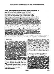
Fig. 2. A symmetric hierarchy: (a) schema and (b) examples of instances.
Symmetric spatial hierarchies have at the schema level only one path where all levels are mandatory. An example is given in Figure 2. At the instance level the members form a tree where all the branches have the same length. As implied by the cardinalities, all parent members must have at least one child member and a child member cannot belong to more than one parent member. Asymmetric spatial hierarchies have only one path at the schema level (Figure 3) but, as implied by the cardinalities, some lower levels of the hierarchy are not mandatory. Thus, at the instance level the members represent a nonbalanced tree, i.e., the branches of the tree have different lengths. The example of Figure 3 represents an asymmetric spatial hierarchy for a forest division consisting of little cell, cell, segment, and region. Since some parts of the forest are located in the mountain and are difficult to access, detailed representations of all areas are not available for analysis purposes and some hierarchy members are leaves at the segment or at the cell levels. Generalized hierarchies contain multiple exclusive paths sharing some levels (cf. Figure 4). All these paths represent one hierarchy and account for the same analysis criterion. At the instance level each member of the hierarchy belongs to only one path. The symbol ⊗ indicates that for every member the paths are exclusive. In the example it is supposed that road segments can belong to either city roads or to highways, where the management of city roads is the responsibility of districts while that of highways is privatized. Notice that the geometry associated to the Company level (a simple area) represents the spatial extent that a company is responsible for maintenance.
Little cell
Cell
Segment
Region
Id Access condition Type Size Other attributes
Id Size Description Other attributes
Id Size Responsible Other attributes
Id Name Other attributes
a) region X segment 1 cell 11 little cell 111
segment 2
cell 12
segment 3
cell 31
cell 32
cell 33
b)
little cell 112
Fig. 3. An asymmetric spatial hierarchy: (a) schema and (b) examples of instances. District Road Segment Number Speed limit Condition Other attributes
City
Name Responsible Other specific attributes
X
Name Area Other specific attributes
State X Name Area Other specific attributes
Company Name Address Other specific attributes
a) state A city X district 1
company 1
city Y
company 2
district 2 road segment 21
road segment h21
road segment 22
road segment h22
b) Fig. 4. A generalized spatial hierarchy: a) schema and b) examples of instances.
As another example, the data model of the U.S. Census-Administrative Boundaries [16] includes several generalized hierarchies. One of them represents a spatial hierarchy containing a county level. However, in Maryland, Missouri, Nevada, and Virginia the county level is replaced by independent cities or places, whereas in American Samoa, county is replaced by district and islands.
3.2
Non-strict spatial hierarchies
Until now we have assumed that the parent-child links have one-to-many cardinalities, i.e., a child member is related to at most one parent member and a parent member may be related to several child members. However, many-tomany cardinalities are very common in real-life applications: e.g., a mobile phone network cell may belong to several ZIP areas [4], several tribal subdivisions in the U.S. Census hierarchy belong both to the American Indian reservation and to the Alaska Native areas [16]. We call a spatial hierarchy non-strict if it has at least one many-to-many cardinality; it is called strict if all cardinalities are one-to-many. The members of a non-strict hierarchy form a graph. The fact that a hierarchy is strict or not is orthogonal to its type. Thus, the different kinds of hierarchies already presented can be either strict or non-strict.
State
Lake
City
Name Length Pollution level Other attributes
City name City population Other attributes
a)
State name State population State area State major activity Other attributes
state A city 1
city 2
city 3
lake X
lake Y
b) Fig. 5. A symmetric non-strict hierarchy: (a) model and (b) example of instances.
Figure 5 shows a symmetric non-strict spatial hierarchy. The many-to-many cardinality represents the fact that a lake may belong to more than one city. This hierarchy may be used, e.g., for controlling the lake contamination level caused by neighbour cities. Most non-strict hierarchies arise when a partial containment relationship takes place [4], e.g., when only part of a highway belongs to a state. In real situations it is difficult to find non-strict hierarchies with a full containment relationship, i.e., when a spatial member of a lower level wholly belongs to more than one spatial member of a higher level. 3.3
Multiple alternative spatial hierarchies
Multiple alternative spatial hierarchies have several non-exclusive simple spatial hierarchies sharing some levels. However, all these hierarchies account for the
same analysis criterion. At the instance level such hierarchies form a graph since a child member can be associated with more than one parent member belonging to different levels. In multiple alternative spatial hierarchies, it is not semantically correct to simultaneously traverse the different composing hierarchies: The user must choose one of the alternative hierarchies for analysis.
Census Block Number Other attributes
Tribal Block Group Number Other attributes
County
State
Name Other attributes
Name Other attributes
Tribal Census Tract Number Other attributes
Tribal Census Subdivision
American Indian Reservation
Number Other attributes
Name Other attributes
Nation Name Other attributes
Fig. 6. Multiple alternative hierarchies formed by two non-strict symmetric hierarchies.
The example given in Figure 6 represents part of the hierarchies used in the U.S. Census Bureau [16]. The hierarchy for American Indian and Alaska Native Areas, and Hawaii Home Land (AIANA/HHL) uses a particular subdivision of the territory (lower path of the figure). However, the usual hierarchy composed, among others, of County and State levels1 (upper path of the figure) provides another subdivision of the same territory. This path can be used for obtaining statistics of American Indian by counties and states. It is obvious that both hierarchies cannot be simultaneously used during analysis. Notice the difference between generalized and multiple hierarchies (Figures 4 and 6). Although both hierarchies share some levels and use only one analysis criterion, they represent different situations. In a generalized hierarchy a child member is related to one of the paths, whereas in multiple hierarchies a child member is related to all paths, and the user must choose one of them for analysis. 3.4
Parallel spatial hierarchies
Parallel spatial hierarchies arise when a dimension has associated several spatial hierarchies accounting for different analysis criteria. Such hierarchies can be independent or dependent. In a parallel independent spatial hierarchy, the different hierarchies do not share levels, i.e., they represent non-overlapping sets of hierarchies. An example is given in Figure 7. In contrast, parallel dependent spatial hierarchies, have different hierarchies sharing some levels. The example in Figure 8 represents an insurance company that includes hospitalization services for clients. The Client dimension contains two hierarchies: a symmetric hierarchy representing the hospitalization structure and a non-covering one representing the geographic division of the client’s address. Both hierarchies share the common levels of City and State. Notice that 1
To simplify the example, we ignore that some states are not divided in counties.
Store
City
State
Region
Store number Store name Store address Other attributes
City name Other attributes
State name Other attributes
Region name Other attributes
Sales group district
Sales group region
District name Other attributes
Region name Other attributes
Fig. 7. Parallel independent spatial hierarchies associated to one dimension.
the difference between multiple alternative and parallel dependent hierarchies (Figures 6 and 8) consists in allowing one or several analysis criteria.
Client Id First name Last name Middle name Address Other attributes
Hospitalization Area
Hospitalization Region
Area name Other attributes
Region name Other attributes
Symmetric hierarchy
Hospital. Municipality Municip. name Other attributes
City City name Other attributes
County X
State
County name Other attributes
X
State name Other attributes
Non-covering hierarchy
Fig. 8. Parallel dependent spatial hierarchies.
4
Topological relationships between spatial levels
As already said, the levels related by a child-parent relationship may be spatial or non-spatial. This leads to 4 possible combinations: non-spatial-to-non-spatial (the child and parent levels are thematic), spatial-to-non-spatial (a spatial level rolls-up to a non-spatial level), non-spatial-to-spatial (a non-spatial level rolls-up to a spatial level), and spatial-to-spatial (both levels are spatial). To each one of these combinations corresponds a different relationship type: (1) a containment function for non-spatial-to-non-spatial relationships, (2) a mapping from a spatial to a non-spatial domain for spatial-to-non-spatial relationships, (3) a mapping from a non-spatial to a spatial domain for non-spatial-to-spatial relationships, and (4) a topological relationship for spatial-to-spatial relationships. The first kind of relationship has been widely investigated. Mappings from spatial to non-spatial domains (or vice versa) can be easily implemented. The question that remains is which kinds of topological relationships should be allowed between spatial levels considering that these hierarchies are used for aggregating measure values when traversing levels.
While topological relationships between hierarchy levels are the focus of much research (e.g., [15]), few works relate these relationships to the problem of measure aggregation [11, 4]. For non-spatial hierarchies, summarizability conditions [6] must hold for ensuring the correct aggregation of measures in higher levels taking into account existing aggregations in lower levels. These conditions include, among others, a simple-value mapping between hierarchy levels and completeness (i.e., no missing values and existence of a parent member for every child member). Since asymmetric, generalized, and non-strict hierarchies do not satisfy summarizability conditions, it is required to apply either special aggregation procedures (such as those implemented in Microsoft Analysis Services [9] for asymmetric and non-covering hierarchies), or transformations such as those described in [4] for asymmetric, non-covering, and non-strict hierarchies. Although the summarizability conditions have been established for non-spatial hierarchies they must also hold for spatial hierarchies. However, summarizability problems may also arise depending on the topological relationship existing between spatial levels. Several solutions may be applied: an extreme one is to disallow the topological relationships that cause problems whereas another solution is to define customized procedures for ensuring correct measure aggregation. We give next a classification of topological relationships2 according to the required procedures for establishing measure aggregation. Our classification, shown in Figure 9, is based on the intersection between the geometric union of the spatial extents of child members (denoted by GU (Cext )) and the spatial extent of their associated parent member (denoted by Pext ). To simplify the discussion, we only consider spatial hierarchies with distributive numeric measures, e.g., sum3 . Forbidden Topological relationship
Disjoint
disjoint
Related
Total containment
Equal
within
equal Boundary touches
Safe aggregation Special aggregation procedure Connected
Interior crosses for curves
Both crosses overlaps
Fig. 9. Classification of topological relationship for aggregation procedures.
The disjoint topological relationship is not allowed between spatial hierarchy levels since during a roll-up operation the next hierarchy level cannot be reached. Thus, a non-empty intersection between GU (Cext ) and Pext is required. 2 3
We consider the topological relations from the SQL/MM standard [3]. We do not consider spatial measures obtained by applying spatial operators or functions to spatial objects [8] as proposed by [11].
Different topological relationship may exist if the intersection of Pext and GU (Cext ) is not empty. If GU (Cext ) within Pext , then the geometric union of the child member extents (as well as the extent of each child member) is included in their parent member extent. In this case the aggregation of measures from a child to a parent level can be done safely using a traditional approach. Similar situation occurs if GU (Cext ) equals Pext with the additional constraint that both spatial extents are equal and have common boundaries. The situation is different if the extents of child and parent members are related by a topological relationship distinct from within or equal. As can be seen in Figure 9 different topological relationships belong to this category, e.g., touches, crosses. As in [12], we distinguish three possibilities depending on whether a topological relationship exists between the boundaries, the interiors, or both the boundaries and the interiors of the spatial extents of child and parent members. For example, this distinction is important in Figure 8 for determining how to realize aggregations if a lake touches a city and overlaps another. When developing aggregation procedures, if GU (Cext ) intersects Pext and this intersection is different from equal or within, the spatial extent of some (or all) child members is not completely included in the spatial extent of a parent member. The topological relationship existing between the spatial extents of individual child members and a parent member determines which measure values can be considered in its entirety for aggregation and which must be partitioned. For example, if in the hierarchy in Figure 2 the geographic union of the points representing stores is not within the spatial extent of their county, every individual store must be analyzed for determining how the measure (for example, required taxes) should be distributed between two or more counties. Therefore, an appropriate procedure for measure aggregation according to application particularities must be developed, such as that proposed by [4] for partial containment topological relationship. As already said, another solution is to disallow these topological relationships in spatial hierarchies.
5
Related work
Many works focus on conceptual modelling for Spatial Databases (e.g., [10]) or for DWs (e.g., [14]) based on either the ER model or the UML. However, a multidimensional model is seldom used for spatial data modelling. Moreover, even though organizations such as ESRI recognize the necessity of conceptual modelling by introducing templates of spatial data models in different areas of human activities [1], these models often refer to particular aspects of the logicallevel design and are too complex to be understood by decision-making users. Ferri et al. [2] refer to common key elements between spatial and multidimensional databases: time and space. They formally define a geographic data model including contains and full-contains relationships between hierarchy levels. Based on these relationships, the integration between GIS and DW/OLAP environments can be achieved by a mapping between the hierarchical structures of both environments. The concept of mapping between hierarchies is also
exploited by Kouba et al. [5]. To ensure the consistent navigation in a hierarchy between OLAP systems and GISs, they propose a dynamic correspondence through classes, instances, and action levels. Stefanovic et al. [13] distinguish three types of spatial dimensions based on the spatial references of the hierarchy members: non-spatial (a traditional nonspatial hierarchy), spatial-to-non-spatial (a spatial level rolls-up to a non-spatial level), and fully spatial (all hierarchy levels are spatial). Jensen et al. [4] present a general scenario for location-based services (LBSs) including a data warehouse as central storage platform. Their model includes several dimensions, one of which is a spatial dimension. They proposed a model with hierarchies including a new partial containment relationship where only part of the spatial extent of a member belongs to a higher hierarchy level. Although the works mentioned above refer to spatial hierarchies in DW and/or OLAP, only [4] classify spatial hierarchies. However, they neither include generalized hierarchies nor distinguish partly and fully spatial hierarchies. Further, since they do not focus on the graphical representation of the different kinds of hierarchies, some of them are difficult to distinguish, e.g., non-covering and multiple hierarchies. The work of Pedersen and Tryfona [11] refers to pre-aggregation in spatial DWs. However, we consider that the analysis they present and the solution they proposed are adequate for managing spatial measure represented by geometry [8] and it goes out of the scope of this article.
6
Conclusions
DW and OLAP systems use a multidimensional model for representing user requirements for decision making. In this model hierarchies allow to view data at different levels of detail using roll-up and drill-down operations. On the other hand, Geographic Information Systems (GISs) have been successfully used for many years in a great number of applications areas. Since it is estimated that 80% of the data stored in databases has a spatial component, the merging of both technologies, DWs and GISs, provides an opportunity to enhance the decisionmaking process. However, the lack of a conceptual approach for multidimensional modeling, joined with the absence of a commonly-accepted conceptual model for spatial applications, makes that representing real-world hierarchies including spatial levels is a challenging task. We extended the different kinds of hierarchies proposed in [7] by the inclusion of spatial levels. Hierarchies may be fully or partly spatial depending on whether all their levels are spatial. Combining spatial and non-spatial levels leads to different relationships between hierarchy levels. Finally, we addressed the summarizability problem that arises for some types of hierarchies indicating the solutions that may be applied in such situations. We emphasized that the summarizability problem may also occur due to the different topological relationships existing between hierarchy levels. We classify these relationships according to the complexity required for developing procedures for measure aggregation.
The present work belongs to a larger project aiming at developing a conceptual model for spatio-temporal data warehouses. We are currently working on the inclusion of temporal features in our model.
References 1. ESRI, Inc. ArcGIS data models. http://www.esri.com/software/ arcgisdatamodels/index.html, 2004. 2. F. Ferri, E. Pourabbas, M. Rafanelli, and F. Ricci. Extending geographic databases for a query language to support queries involving statistical data. In Proc. of the 12th Int. Conf. on Scientific and Statistical Database Management, pages 220–230, 2000. 3. ISO. SQL multimedia and application packages - part 3: Spatial. Technical report, ISO/IEC FCD 13249-3:2003, 2002. 4. C. Jensen, A. Klygis, T. Pedersen, and I. Timko. Multidimensional data modeling for location-based services. VLDB Journal, 13(1):1–21, 2004. 5. Z. Kouba, K. Matouˇsek, and P. Mikˇsovsk´ y. Novel knowledge discovery tools in industrial applications. In Proc. of the Workshop on Intelligent Methods for Quality Improvement in Industrial Practice, pages 72–83, 2002. 6. H. Lenz and A. Shoshani. Summarizability in OLAP and statistical databases. In Proc. of the 9th Int. Conf. on Scientific and Statistical Database Management, pages 132–143, 1997. 7. E. Malinowski and E. Zim´ anyi. OLAP hierarchies: A conceptual perspective. In Proc. of the 16th Int. Conf. on Advanced Information Systems Engineering, pages 477–491, 2004. 8. E. Malinowski and E. Zim´ anyi. Representing spatiality in a conceptual multidimensional model. In Proc. of the 12th ACM Symposium on Advances in Geographic Information Systems, pages 12–21, 2004. 9. Microsoft Corporation. SQL Server 2000. Books Online. http://www.microsoft. com/sql/techinfo/productdoc/2000/books.asp, 2003. 10. C. Parent, S. Spaccapietra, and E. Zim´ anyi. Spatio-temporal conceptual models: Data structures + Space + Time. In Proc. of the 7th ACM Symposium on Advances in Geographic Information Systems, pages 26–33, 1999. 11. T. Pedersen and N. Tryfona. Pre-aggregation in spatial data warehouses. In Proc. of the 7th Int. Symposium on Advances in Spatial and Temporal Databases, pages 460–478, 2001. 12. R. Price, N. Tryfona, and C. Jensen. Modeling topological constraints in spatial part-whole relationships. In Proc. of the 20th Int. Conference on Conceptual Modeling, pages 27–40, 2001. 13. N. Stefanovic, J. Han, and K. Koperski. Object-based selective materialization for efficient implementation of spatial data cubes. IEEE Trans. on Knowledge and Data Engineering, 12(6):938–958, 2000. 14. N. Tryfona, F. Busborg, and J. Borch. StarER: A conceptual model for data warehouse design. In Proc. of the 2nd ACM Int. Workshop on Data Warehousing and OLAP, pages 3–8, 1999. 15. N. Tryfona and M. Egenhofer. Consistency among parts and aggregates: a computational model. Transactions in GIS, 4(3):189–206, 1997. 16. U.S. Census Bureau. Standard Hierarchy of Census Geographic Entities and Hierarchy of American Indian, Alaska Native, and Hawaiian Entities. http: //www.census.gov/geo/www/geodiagram.pdf, 2004.