Spatial memory of paths using circular probability

Spatial memory of paths using circular probability distributions: Theoretical properties, navigation strategies and orientation cue combination Julien Diard, Pierre Bessière and Alain Berthoz Laboratoire de Psychologie et NeuroCognition, CNRS, Grenoble, France and Laboratoire de Physiologie de la Perception et de l’Action, CNRS / Collège de France, Paris, France Abstract We propose a mathematical model of the Path Integration (PI) process. Its core assumption is that orientations of a path are summarized by circular probability distributions. We compare our model with classical, deterministic models of PI and find that, although they are indistinguishable in terms of information encoded, the probabilistic model is more parsimonious when considering navigation strategies. We show how sensory events can enrich the probability distributions memorized, resulting in a continuum of navigation strategies, from PI to stimulus-triggered response. We analyze the combination of circular probability distributions (e.g., multi-cue fusion), and demonstrate that, contrary to the linear case, adding orientation cues does not always increase reliability of estimates. We discuss experimental predictions entailed by our model.

This paper is concerned with mathematical modeling of the Path Integration (PI) process. More precisely, we are interested in the way global spatial properties of a path can be estimated and used by a navigator. Here, we use the word navigator as a general term to encompass both simulated and real moving entities, whether they are natural or artificial. A classical example of the purpose of PI is when a navigator is interested in estimating the angle and distance between a starting and ending point of a path, in order to be able to go back to the starting point of this path, using a shortcut trajectory. Several reviews already presented the variety of mathematical definitions of possible PI mechanisms (Benhamou & Séguinot, 1995; Etienne & Jeffery, 2004; Maurer & Séguinot, 1995; Merkle, Rost, & Alt, 2006; Vickerstaff & Cheung, 2010). In particular, the two most recent of these classify PI models according to the reference frame used in the computations

This work has been supported by the BACS European project (FP6-IST-027140). Authors wish to gratefully acknowledge stimulating help from Panagiota Panagiotaki and Matthieu Lafon, and insightful comments from the anonymous reviewers.

PATH MEMORIZATION USING CIRCULAR PROBABILITY DISTRIBUTIONS

2

(either geocentric – i.e. allocentric – or egocentric) and the vector basis used for encoding displacements (either polar or Cartesian). We summarize the four principal models we wish to highlight, in order of historical appearance. The first mathematical formulation of PI is attributed to Jander (1957). In this model, the final estimate of angles is a simple average of experienced angles, which, unfortunately, is not correct geometrically. Indeed, the first geometrically correct model is the bi-component model (Mittelstaedt, 1962; Mittelstaedt & Mittelstaedt, 1982), as it estimates two components to recover the XE , YE position of the end-point E of the path by:

XE =

N X i=0

cos(θi ), YE =

N X

sin(θi ) ,

(1)

i=0

where θ0 , θ1 , . . . , θN is the sequence of angles experienced along a path. From these two coordinates, recovering the global angle Φ and distance D is straightforward. M¨ uller and Wehner then developed a variant of the initial model of Jander to allow a recurrent estimation process in an egocentric reference frame (M¨ uller & Wehner, 1988). To do so, they dropped the geometrical correctness in favor of neurocomputational plausibility, and proposed an approximate estimation process, further modified to better fit experimental data (introducing empirically determined constants, for instance). Finally, a recent paper by Vickerstaff and Cheung (2010) develops mathematical formulations of PI for various reference frames, leading to elegant differential equations for updating processes and a complete translation scheme between reference frames, to discuss the mathematical (lack of) distinguishability of the considered formulations. Several variants are noteworthy, and highlight the complexity and richness of PI processes. What is the influence, for instance, of random errors in the estimation of elementary displacements (Benhamou, Sauvé, & Bovet, 1990)? How can angles and distance be estimated while following a non-discretized, continuous path? Is this updating process itself continuous (Gallistel, 1990; Merkle et al., 2006)? If it is discrete, does it need to be sampled regularly over time or space? Or, in other words, does the step length need to be constant (Benhamou, 2004)? Going beyond purely motor inputs to the PI process, how do other sensory modalities contribute to PI estimations (Etienne, Maurer, & Séguinot, 1996; Etienne & Jeffery, 2004)? Does tracking multiple goals or starting locations over time require several PI processes, or a single one that would be reset? How about tracking multiple spatial relations simultaneously (Biegler, 2000)? Whatever the extension considered, a common assumption to previous models is that PI would be concerned with the computation of values, like angles or distances. Indeed, in textbook presentations of PI (Batschelet, 1981; Jammalamadaka & SenGupta, 2001), the mean vector is usually presented as the correct summary of a trajectory, which is very close to the bi-component model above. Indeed, the mean vector has the same direction as the vector sum of N elementary displacements, i.e., tan Φ = YE /XE . Let D be the length of the vector sum of N elementary displacements; the mean vector length is, by definition, D/N .


3

Bayesian encoding of spatial relations The core of our approach is to assume that uncertainties are incorporated as a central component of the memory system. In this view, states of knowledge about the sensorimotor interactions with the environment are not encoded by single values, but by probability distributions. This is a subjectivist approach to probabilities: probability distributions encode states of knowledge of individual subjects (Colas, Diard, & Bessière, 2010; Jaynes, 2003). In this paper, we therefore use the term Bayesian in this specific sense 1 . In life sciences, the assumption that probability distributions might be assessed and manipulated by sensorimotor systems is gaining momentum, concerning both the encoding of single quantities and the combination of several quantities. In this last case, this is the now classical model of statistically optimal fusion for perception, that was applied to various cases of intramodal cue fusion (Drewing & Ernst, 2006; Hillis, Watt, Landy, & Banks, 2004; R. A. Jacobs, 1999) and multimodal sensory fusion, both in cases of congruent (Anastasio, Patton, & Belkacem-Boussaid, 2000; Körding & Wolpert, 2004; Zupan, Merfeld, & Darlot, 2002) and conflicting cues (Alais & Burr, 2004; Banks, 2004; Battaglia, Jacobs, & Aslin, 2003; Ernst & Banks, 2002). Memorizing orientations using von Mises probability distributions Returning to the specific case of PI modeling, we reformulate our central question. Let us assume a PI system based on a probabilistic model of the orientations experienced along a trajectory: what are its properties? What is the difference, if any, between such a probabilistic PI model and a deterministic PI model? What information would be stored? What would be the properties of resulting navigation strategies and their combination? How could a probability distribution over orientations be combined with other sources of information? To study these questions, we first introduce a Bayesian formulation of a Path Integration process, based on circular probability distribution, i.e., probability distributions that behave mathematically correctly over the discontinuity of circular spaces at −π. We consider unimodal distributions, that is to say, bell-shaped, “Gaussian-like” distributions over circular spaces. The mathematical tool we choose here is von Mises probability distributions, whose parameters are a preferred direction µ and some measure of the confidence about this direction, in the form of a concentration parameter λ. There are four main results to our analysis. • The first result is an indistinguishability result. We study the properties of the µ and λ parameters: µ acts as an estimate of the angle to the base, and λ helps retrieve the distance to the base, relative to the travelled distance. In other words, the λ parameter turns out to be both a measure of the variability of angles and a distance estimate. It leads to a an internal representation which explicitly encodes the direction to the starting point S of the path, and implicitly encodes the distance to S. Our first result concerns the comparison of the probabilistic model of PI based on von Mises probability distributions and the deterministic model of PI based on mean vectors: both encode information of the 1 As opposed to a sense which is more widespread in physics and statistics, for instance, where a model can be said to be Bayesian if it incorporates a non-uniform prior probability distribution.


4

same nature (an angle and D/N ). Therefore, they are indistinguishable in this regard; discriminating them then requires further consideration. • The second and third results both mainly concern the parsimony of our model. Using our probabilistic representation of experienced orientations, we define a single navigation strategy, and show that it yields homing, trajectory-reproduction, or random exploration behaviors, depending on the actual parameters of the learned probability distribution. In other words, in our framework, these strategies do not need to be assumed to be different entities, activated by a hypothetical higher-level arbiter. Instead, they are particular cases over a continuum of navigation strategies, described by varying parameters µ, λ. Moreover, when studying how sensory events enrich the probabilistic representation of orientations, a similar result ties Path Integration and stimulus-driven navigation (route following). They both appear as extremes on a gradual scale of navigation strategies. Indeed, PI summarizes the global spatial properties of a path, whereas route following builds upon a more precise path description, indexed by sensory events. We show how Bayesian inference links the two. These two results also yield discriminating experimental predictions, which we outline. • Finally, the fourth result is a quantitative experimental prediction. We show that, in the context of sensor fusion, the mathematics of probabilistic fusion over circular space are not the same as for linear space. Contrary to the linear case, cue combination in circular spaces does not always increase confidence. This provides a discriminating experimental prediction in order to assess whether spatial quantities are encoded in linear or circular representations in the central nervous system. The rest of the paper is organized as follows. We first recall the definition of von Mises probability distributions, some of their properties and the way their parameters can be identified from experimental data, using a Maximum Likelihood estimation procedure. Next, we apply this parameter estimation procedure to the special case where the orientations used as experimental data come from following a path, and analyze the properties of the resulting probability distribution. We then show how it can be the basis for navigation behaviors, like homing and path reproduction, and how it can serve as a scaffold for anchoring sensory cues observed along the path. Finally, we consider the case of multi-cue fusion in the context of von Mises probability distributions.

von Mises probability distributions Definition Intuitively, von Mises probability distributions are “Gaussian probability distributions over orientations”. In other words, they are unimodal symmetrical probability distributions. However, contrary to Gaussian probability distributions, which are strictly defined over IR, von Mises probability distributions are defined over circular spaces. Applied to a set of angular or orientation data, they allow summarizing it by a preferred angle µ and a concentration λ around that preferred angle. Although the preferred angle µ can be thought of as the equivalent of an “average angle”, the concentration parameter behaves in an opposite manner from standard-deviations: as λ grows, the von Mises distribution gets more and more peaked. The probability density function, denoted vM, of a von Mises distribution is given by (Abramowitz & Stegun, 1965; Batschelet, 1981; Dowe, Oliver, Baxter, & Wallace, 1995;


5

Shatkay & Kaelbling, 1998): P (θ | µ λ) = vM(θ; µ, λ) =

1 eλ cos(θ−µ) , 2πI0 (λ)

(2)

with µ ∈ [−π, π), λ ≥ 0, and where I0 (λ) is the modified Bessel function of the first kind and order 0 (Shatkay & Kaelbling, 1998), defined as: I0 (λ) =

∞ X 1 λ 2r r=0

r!2

2

,

(3)

or, alternatively (Abramowitz & Stegun, 1965; Fu, Chen, & Li, 2008): 1 I0 (λ) = π

Z π

λ cos(θ)

e 0

1 dθ = π

Z π

cosh(λ cos(θ)) .

(4)

0

I0 (λ) cannot be computed in closed form (Abramowitz & Stegun, 1965); it will therefore be assumed in the following that von Mises probability distributions are computed as P (θ | µ λ) = eλ cos(θ−µ) and normalized numerically afterwards. A couple of limit cases need attention. On the one hand, when λ = 0, and since I0 (0) = 1, the probability density function (2) becomes: ∀µ ∈ [−π, π), P (θ | µ [λ = 0]) =

1 . 2π

(5)

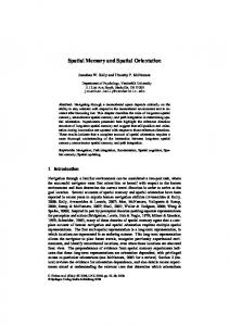
In other words, when the concentration parameter λ is 0, the von Mises probability distribution degenerates to a uniform probability distribution over all possible angles, and the value of the preferred direction µ becomes undefined. For this reason, some references (Shatkay & Kaelbling, 1998) restrict the range of λ to strictly positive real values: λ > 0. On the other hand, at the other extreme, when λ gets larger, von Mises probability distributions get more peaked, so that they converge towards Dirac delta probability distributions centered on µ, the preferred direction (Jones & Pewsey, 2005). Some examples of von Mises probability distributions over the range [−π, π) are shown Figure 1. As a final introductory note, it should be noted that a recent mathematical treatment by Jones and Pewsey (2005) has shown that von Mises probability distributions could be cast into a large family of distributions over circular spaces. In this family, von Mises, wrapped Cauchy, Cardioid, circular uniform, and Dirac delta (but not wrapped Gaussian distribution) are special cases in a continuum of probability distributions. Out of these so-called “JP distributions”, the von Mises, wrapped Cauchy and Cardioid probability distributions are circular, unimodal and symmetrical. Most of the properties we discuss in this paper derive from these properties. Therefore, although we center our study on von Mises distributions, it is very likely that our results generalize to other probability distributions of this family and to wrapped Gaussian distributions, although with different mathematical treatments. Maximum Likelihood parameter estimation for von Mises distributions Let ∆ = {θi }N i=1 be a set of N experimental data, each θi being an angle expressed in radians. We look for the parameters µ, λ of maximum likelihood, given the data ∆. The

6


Π 2

0.6

3Π 4

0.6

Π 4

PHΘ È Μ ΛL

0.5 Μ = undef., Λ = 0

0.4

0.4 0.2

Μ = 0, Λ = 3

0.3 0.2

Μ=-

3Π , 4

0

Π

Λ=2

0.1 0.0 -Π

- Π2

0

Π 2

Π - Π4

- 34Π

Θ

- Π2

Figure 1. Examples of von Mises probability distributions for various µ, λ parameter values. Left: von Mises probability distributions are plotted against the [−π, π) interval. Right: the same von Mises probability distributions, plotted on a polar reference frame, using the standard trigonometric convention (0 angle eastward, positive angles counter-clockwise): for λ = 0, this display shows the von Mises as a circle. As λ grows, the distribution gets elongated in the µ direction.

likelihood function is given by: L(µ, λ) = P (∆ | µ λ) = =

N Y

P (θi | µ λ)

i=1 N Y i=1

L(µ, λ) =

(6) (7)

1 eλ cos(θi −µ) 2πI0 (λ) 1

eλ N (2πI0 (λ))

PN i=1

cos(θi −µ)

(8) .

(9)

¯ be the maximum likelihood estimates of µ, λ. Because of I0 (λ), there is no Let µ ¯, λ ¯ However, it is possible to first find an (asymptotically) exact closed form formula for µ ¯, λ. ¯ based on this µ µ ¯ estimate, then estimate λ ¯ estimate (Jones & Pewsey, 2005; Shatkay & ¯ one after the other. Kaelbling, 1998). In other words, we compute µ ¯ and λ Let us first compute the maximum likelihood preferred orientation µ ¯: y¯ µ ¯ = max L(µ, λ) = arctan( ) , µ x ¯ with

PN

PN

y¯ =

i=1 sin(θi )

(10)

and x ¯=

i=1 cos(θi )

. (11) N N ¯ is the solution to (Jammalamadaka & SenGupta, 2001; Shatkay & Kaelbling, Now, λ 1998): N ¯ I1 (λ) 1 X cos(θi − µ) , (12) ¯ =N I0 (λ) i=1 ¯ the modified Bessel function of the first kind and order 1. In general, the with I1 (λ) modified Bessel function of the first kind and order n, for integer values of n, is defined by

7

1.0

1.0

0.8

0.8

0.6

0.6

A1HΛL

A1HΛL


0.4 0.2 0.0

0.4 0.2

0

20

40

60

80

100

0.0 0.001

0.01

Λ

0.1

1

10

100

Λ

Figure 2. Plots of A1 (λ) = I1 (λ)/I0 (λ). Left: linear scale. Right: log-linear scale.

(Abramowitz & Stegun, 1965): In (λ) =

1 π

Z π

eλ cos(θ) cos(nθ)dθ .

(13)

0

In Eq. (12), µ is unknown, so we replace it with the estimated µ ¯. After some trigonometry, ¯ we need to find λ that solves: q ¯ I1 (λ) x ¯2 + y¯2 . (14) = ¯ I0 (λ) This function of λ is usually noted A1 (Codling & Hill, 2005; Fisher, 1993; Jammalamadaka & SenGupta, 2001): A1 (λ) = I1 (λ)/I0 (λ) . (15) A1 has no closed form formula, but can be approximated; it is shown Figure 2. ¯ amounts to inverting the A1 function. There are two main methods for Finding λ this; firstly, there is an approximate form for A−1 1 (Fisher, 1993) A−1 1 (x) =

 3 5   2x + x + 5x /6

x < 0.53 −0.4 + 1.39x + 0.43/(1 − x) 0.53 ≤ x < 0.85   1/(x3 − 4x2 + 3x) x ≥ 0.85

;

(16)

secondly, a more brute force approach consists in building a lookup table (Shatkay & Kael¯ are tried, and the one that is selected bling, 1998). More precisely, some range of values of λ is the one that minimizes: q 2 2 ¯ − x A1 (λ) ¯ + y¯ . (17) Figure 3 shows some examples of results of this estimation process.

Path Integration based on von Mises probability distributions von Mises probability distributions as path summaries The previous section introduced the von Mises probability distributions, and the way their parameters could be estimated, given any data set ∆ of directional data. We now

8

0.7

0.7

0.6

0.6

0.5

0.5 PHΘ È Μ ΛL

PHΘ È Μ ΛL


0.4 0.3

0.4 0.3

0.2

0.2

0.1

0.1

0.0 -Π

- Π2

0 Θ

Π 2

0.0 Π

-Π

- Π2

0

Π 2

Π

Θ

Figure 3. Examples of von Mises probability distributions learned from data. The data are 1000 data points shown as histograms on the [−π, π) interval, with bin counts scaled vertically for readability. The example on the right illustrates the fact that von Mises probability distributions learned from data behave correctly over the −π discontinuity.

turn to the specific case where the observations are paths or trajectories, from which sets of directional data ∆ can be extracted. In this paper, because we focus on the comparison of deterministic and probabilistic models of PI, we set aside some of the extensions we mentioned in the introduction; the initial analysis we propose is restricted to the case of a discretized path, with elementary steps of exactly unit length, etc. We define our notation. Let v be a planar path, decomposed in a discrete manner as a sequence of length N of positions {hxt , yt i}N t=1 . Between consecutive positions, each elementary displacement is of the same length. Path v starts at point S of coordinates xS , yS (assumed, in the following, to be (0, 0) for simplicity, and without loss of generality), and ends at point E of coordinates xE , yE . We reuse here the notation of Benhamou and Séguinot (1995); this is illustrated Figure 4. Given a path v in a plane, a history of elementary angles ∆ = {θt }N t=1 can be obtained by computing, at each position along the path, the angle of the next elementary displacement (or, in the continuous case, this can be approximated by the tangent to the path). Measuring these angles requires an orientation reference frame, i.e., a choice for rotations corresponding to positive angles, and a fixed orientation, noted 0. None of these is constrained by the mathematics of our model. The choice of following trigonometric rotations (positive angles for counter-clockwise rotations), used in the following, is purely arbitrary. Also, the model is agnostic with respect to the nature of the orientation reference; it could refer either to a geocentric cue readily available (position of a distant landmark, e.g., a mountain or the sun), or to a memorized egocentric orientation (e.g., the heading at the start of the trajectory) (Berthoz et al., 1999). How this reference frame is set and updated is beyond the scope of our model; an obvious extension of the model would, of course, be to study the effect of drift of this reference frame, or errors in the memory system that sustains it (noise, decay, etc.). We thus assume that a navigator, having experienced a given path v of length N (its forward trip), observes the orientations ∆ = {θt }N t=1 , and identifies the most likely von Mises probability distribution Pf (θ | ∆). In other words, the forward trip is summarized


9

Y θt

E = (Xt, Yt)

θt-1 (Xt-1, Yt-1)

D S

X

Φ

Figure 4. Schema of path v and associated variables. Path v is approximated by a sequence of positions (Xt , Yt ) joined by discrete segments of angles θt ; the overall relation between S and E, the starting and ending positions of v, is given by beeline distance D and angle Φ.

by an overall direction µf and a concentration around that preferred direction λf : Pf (θ | ∆) = vM(θ; µf , λf ) .

(18)

Figure 5 shows several examples of simulated forward trips, “top-view” polar histograms of the set of angles along these paths and polar displays of the learned von Mises, centered at the final positions of the paths. Geometrical properties of von Mises probability distributions as path summaries In this section, we first show that the parameter µf of the learned von Mises probability distribution is the angle Φ between the starting point S and ending point E of the path. We then demonstrate that the concentration parameter λf has actually the same information content as the distance D between S and E, provided that the length of the path N is known. Firstly, consider the µf parameter. The maximum likelihood estimation (Eq. (10) and (11)) yields: PN

µf = arctan

i=1 sin(θi )/N PN i=1 cos(θi )/N

!

PN

= arctan

i=1 sin(θi ) PN i=1 cos(θi )

!

,

(19)

N provided N 6= 0. Of course, N i=1 sin(θi ) = yE , and i=1 cos(θi ) = xE : these sums of sines and cosines are the coordinates of the end-point of the path in the Cartesian geocentric reference frame. Therefore, taking the arctangent of the ratio yE /xE is indeed computing the angle Φ. Secondly, consider the λf parameter. Eq. (11) and (14) show that:

P

¯ = A1 (λ)

P

q

x ¯2 + y¯2

(20)

10

PATH MEMORIZATION USING CIRCULAR PROBABILITY DISTRIBUTIONS !Μ # 0.645025, Λ # 4.35263"

100 80

Y

Y

60

!Μ # 2.70556, Λ # 0.258371"

80

40

60

30 20

40

Y

!Μ # 0.659091, Λ # 14.9363"

40

10

20 20

0 0

0

!10 !20

0

20

40

60

80

100

120

!20

0

20

40

60

!30

80

!20

X

X

!10

0

10

20

30

X

Figure 5. Examples of Von Mises probability distributions learned from paths. For each, the path is shown in a dashed line starting from (0, 0), while the solid lines are the polar probability distributions of the learned von Mises (parameter values shown on top). Left: a rather straight trajectory leads to a very peaked von Mises. Center: A less direct trajectory that reaches a similar end position has a lower concentration parameter λ, i.e., a higher uncertainty. Right: a trajectory almost completing a circle leads to a very flat von Mises (almost uniform over [−π, π)). s

=

(

PN

2 i=1 cos(θi ))

+( N2

PN

2 i=1 sin(θi ))

(21)

p

= ¯ = A1 (λ)

xE 2 + yE 2 N

D . N

(22) (23)

¯ is the one such that In other words, the concentration parameter of maximum likelihood, λ, ¯ A1 (λ) is equal to the ratio of two distances: D, the shortest distance between S and E, and N , the length of path v actually followed from S to E. Eq. (23) ties the evolution of the λ parameter with D/N , which is called the straightness index (Benhamou, 2004) or the net-to-gross displacement ratio (NGDR) (Bartumeus, Catalan, Viswanathan, Raposo, & da Luz, 2008). Also, recall Eq. (12): N X ¯ = 1 A1 (λ) cos(θi − µ) . N i=1

(24)

This ties the evolution of λ with the orientation efficiency, which is approximated by the mean cosine of directional errors (Benhamou, 2004). At this point, three properties of A1 (λ) = I1 (λ)/I0 (λ) appear to be relevant (Jammalamadaka & SenGupta, 2001): A1 is strictly monotonic and differentiable everywhere, so that it is a bijection, and its range is [0, 1]. This implies, for instance, that λ increases as A1 (λ) increases. This also clarifies the extreme cases. Firstly, this shows that λ = 0 if and only if A1 (λ) = D/N = 0. The learned von Mises degenerates to a uniform probability distribution over angles only if D is zero, i.e., when the travelled path v is a loop and the starting point S and end-point E are superposed. Secondly, it can also be seen that λ tends to large values when A1 (λ) = D/N tends to 1. The learned von Mises gets extremely peaked only if D equals N , i.e., when the travelled path v is a straight line between S and E.


11

Therefore, it can be seen that the concentration parameter λ has two interpretations; it is both a measure of the variability of angles experienced while following the path v, and a measure of the sinuosity of v. When the length N of v is known, λ is actually in bijection with D, the distance between the start and end-point of v. In other words, knowing both the length of the performed trajectory and the variability of experienced orientations provides a unique estimate of the distance to the starting position (by inversion of the A1 (λ) function). Discussion Most species that control their movements in their environment possess various idiothetic information about their displacements, both in translation and rotation. It is therefore safe to assume that both the length of the outward trajectory and variability of orientations can be estimated from egocentric cues. The length of the trajectory is certainly estimated by temporal integration of a combination of estimators (Montello, 1997), like step counting or stride integration (Wittlinger, Wehner, & Wolf, 2006), optic flow (Dacke & Srinivasan, 2007), time elapsed (when speed is somewhat constant), and energy expenditure. Although these last two are debated, and mostly discounted when considering insect navigation (Wolf, 2011), it is known that expected effort biases estimation of distance in humans (Proffitt, Stefanucci, Banton, & Epstein, 2003; Proffitt, 2006). These cues, whatever their combination, would provide an estimate for N , the travelled distance. Observation of orientations is provided by a variety of sensors related with turning angles, even in ants and spiders (Wolf, 2011). The variability of orientations could be approximated by a neural population that would adjust the width of its bell-shaped activity packet. Such a bell-shaped activity is a common assumption in models of head-direction cells (Arleo & Gerstner, 2001; Mittelstaedt, 2000; Samsonovich & McNaughton, 1997; Sharp, Blair, & Cho, 2001; Stringer & Rolls, 2006; Taube & Bassett, 2003). This would provide an estimation for λ, the concentration parameter. If both N and λ are estimated, and since λ and D/N are linked by a one-to-one correspondence, this implies that navigators would also implicitly obtain an estimate of the distance to home D, without further information required. Therefore, with respect to information encoded, our probabilistic model of PI is not distinguishable from a deterministic model based on mean vectors. In both cases, data gathered along a trajectory are summarized by two parameters: an angle and a mean distance for the mean vector model, and an angle and a concentration parameter for the von Mises model. Models differ in the way information is encoded; neurophysiology models, in this regard, would not help discriminate them clearly. Indeed, in models of head-direction cell activity, a “Gaussian-like” bump of activity is maintained in a preferred direction. Whether its width directly encodes a concentration parameter λ or is fixed (and distance is encoded in another population) is rather unclear. With respect to mathematical sophistication, we would argue that the probabilistic model is not more convoluted than the deterministic model. For instance, the Bessel function appearing in the probability density function formulation never needs to be explicitly computed; indeed, as it appears at the denominator, it can always be replaced by a normalization term. Also, lateral inhibitions in neural ensembles are a possible mechanism for normalizing activity. In the same vein, the A and A−1 functions are non-linear functions.


12

Along the cos and sin functions, which are used in both models, we have to assume that they could be at least approximated by neural computation. This opens up the discussion about a mechanism for incrementally updating the von Mises parameters as individual θi arrive. Mathematical derivations above provide an existence proof of such a mechanism. Indeed, Eq. (10) and (11) can be combined to update the µ parameter on the one hand, and Eq. (20) to (23) to update the λ parameter on the other hand. However, care must be taken not to interpret such a mechanism at face value, as it would suggest that, underlying the probabilistic model, the “true”, “explicit” information to be memorized and updated is the x, y position of the navigator. This would not be a logical consequence: that the existence proof of the update mechanism explicitly uses the x, y quantity does not imply that all update mechanisms do. For instance, there could be a closed form solution to compute new µ, λ as θi arrives that we have not found. Or, a neurological implementation of the update mechanism might very well approximate the updating function. Or, it might also be the case that the probabilistic representation of orientations and its parameters are the “true” information memorized and updated, and that they are used to recover the x, y estimates in some species, when needed. At this point, there are no theoretical grounds on which to discriminate these possibilities. This is a direct consequence of the indistinguishability highlighted above, in terms of information content, between the probabilistic and deterministic model. Another issue that warrants discussion is, of course, noise. The initial development we proposed so far is noise-free. For instance, at each time step, the observed angular displacement θi is assumed to be correct. In a realistic case, this is obviously not the case. Again, because of the indistinguishability we have demonstrated between the probabilistic model and the deterministic model, the impact of noise is, at least qualitatively, well understood: either some stable allocentric cue (sky polarization, sun position, distant visual landmark, etc.) is available, that can be used to recalibrate, so that errors at each time step are corrected and therefore uncertainty in the probabilistic model would be increased by sensory uncertainty, or there is no such cue available, in which case errors will accumulate over time, unbounded. This is the classical distinction between purely idiothetic and allothetic navigation (Cheung & Vickerstaff, 2010), also found in many other domains, like odometry computation in robotics and dead reckoning in maritime navigation. Going further and precisely quantifying the effect of noise on the probabilistic orientation model would require precise hypotheses about sensory noise characteristics, relative frequency of probability distribution updating and recalibration, possible drift of geocentric cues over long time-scales (sun vs. distant mountain), species considered, etc. This is beyond the scope of this general introduction to spatial memorization of paths using circular probability distribution. We have also so far assumed a fixed, unitary step length. Here again, enriching the model by considering variable but perfectly known step length is rather straightforward. However, analyzing the effect of noise about step length would again require precise hypotheses about noise characteristics, geometry of the navigator locomotion apparatus and terrain, whether sensory estimates of elementary displacement are used in conjunction with proprioception and motor efferent copy, which species is considered, etc. This is also beyond the scope of the analysis proposed here. Overall, the theoretical indistinguishability between the deterministic and probabilis-


13

tic models implies that the von Mises model cannot be dismissed on purely conceptual grounds. As an aside, we note that this general topic, i.e., the question of constraints of probabilistic models, and thus their explanatory and predictive power, has been a hotly debated topic for a long time (e.g., see a recent treatment by Jones and Love (2011)). Our strategy, in this regard, is to go beyond theoretical comparison of demonstrably indistinguishable models; in the remainder of this paper, we first examine the parsimony and experimental adequacy of both the deterministic and probabilistic model of PI, and provide discriminating experimental predictions.

Navigation strategies based on probabilistic PI In the deterministic model, a mean vector is assumed to be a summary of traversed paths sufficient to inform navigation strategies. For instance, assuming the navigator is at the starting location, following the mean vector direction orients the navigator towards the end point of the memorized trajectory. On the other hand, if the navigator is at the end position of a trajectory, reversing the mean vector provides a direction toward the starting location. Following this direction thus brings the navigator back to the starting location. A stopping criterion is given by the mean vector length D/N ; if the number of steps N is estimated, it helps recover D, the beeline distance to home. It is quite possible, in the probabilistic model, to perfectly emulate such a navigation strategy. The memorized von Mises probability distribution provides µ, the preferred direction, which can be followed until a stopping criterion based on λ is met (since λ has the same information as D/N , the mean vector length). This would, again, conflate the probabilistic and deterministic model, in terms of predicted trajectories. Therefore, this first navigation strategy is not studied further. Instead, we define another navigation strategy using von Mises probability distributions, with different predictions. The deterministic model predicts that homing trajectories would be straight segments aligned with the homing vector, and that, after a homing trajectory of length D, the navigator would either be exactly back home, or able to engage in a search behavior to, hopefully, find home. Observations deviate from this ideal navigator model. Firstly, in triangle completion tasks, it is commonly observed that navigators do not directly reach home, and instead rally at a point near the beginning of the outward journey. Such errors can be attributed either to systematic underestimations of rotations, to limited memory, or even to the favorable property that crossing the outward journey increases the likelihood of encountering familiar landmarks (Merkle et al., 2006). Such accounts would equally apply both to the deterministic and probabilistic models, and thus would not help discriminate them. Secondly, it is also observed that homing trajectories are not perfectly straight segments (Collett & Collett, 2000; Maurer & Séguinot, 1995; M¨ uller & Wehner, 1988). Humans appear as an exception in this regard, with very straight trajectories in small-scale triangle completion tasks. Most non-human animals will home following somewhat tortuous trajectories. This is even the case when the homing behavior is a result of a startling stimulus (e.g. rattling keys to make a sudden loud noise in gerbil experiments), and thus, quick, optimal, straight ahead fleeing trajectories would be expected (Siegrist, Etienne, Boulens, Maurer, & Rowe, 2003). These deviations are often explained away either by uncontrolled terrain variations (e.g. in return trip of desert ants), uncontrolled sensory input during the


14

homing trajectory (i.e., the observed behavior is not a pure homing behavior), or even to noise in the locomotion and trajectory following processes. Here, we assume that some portion of the observed sinuosity and some of the variability between different trials or different animals are not the result of uncontrolled factors outside of the PI mechanism. Instead, they could also be a direct translation of the concentration parameter of the learned von Mises probability distribution. Indeed, if we assume that a probability distribution is the memorized summary of a path, it seems appropriate to use the full information at hand in subsequent navigation strategies. Consider briefly the alternative: assume that only the µ parameter was used, or, equivalently, that the navigator always follows the most probable direction µ. That would amount to discarding the λ parameter, i.e., half of the memorized information, and would again conflate the trajectories predicted by probabilistic and deterministic models. Therefore, in the following, we explore navigation strategies in which orientations are drawn at random, according to the probability distribution at hand. This randomness directly explains away the variability between trials or animals; even with the same memory state, navigation would never result in the exact same trajectory. We assume that the navigator is capable of “inverting” the learned distribution over orientations. This means that, from Pf (θ | ∆) that represents the probabilities of orientations of the forward trip, the navigator computes Pr (θ | ∆), which is an estimate of the orientations to follow on the return trip. We assume this is done by “flipping” the µf of the learned von Mises distribution by π (i.e., adding 180◦ to µf ), and leaving λf unchanged: µr = µf + π mod 2π

(25)

λr = λf

(26)

Pr (θ | ∆) = vM(θ; µr , λr ) .

(27)

This simple computation can be seen as the equivalent, in the probabilistic setting, of the computation of the opposite vector −~a of vector ~a. Once this reversal is done, directed navigation behaviors are obtained if the navigator draws, at each time step, orientations to follow according to the obtained von Mises probability distribution. Figure 6 shows examples of trajectories obtained by such a sampling process. Not only is the preferred direction µ used as a drive in a given direction, but the concentration parameter λ is translated in the resulting trajectories as well. When λ is large, the trajectories obtained are fairly straight in the µ direction, whereas when λ is small, the drawn directions to follow are more widespread, resulting in more sinuous, less directed trajectories. Note the special case when λ = 0, where von Mises probability distributions degenerate to uniform distributions: the resulting navigation strategy is mathematically exactly a simple isotropic random walk (SRW) (Codling, Plank, & Benhamou, 2008). Updating the homing direction along the return trip Homing behaviors can be built upon the previous mechanism. We assume that orientations are drawn according to the probability distribution pointing home, i.e., Pr (θ | ∆), providing some angle θN +1 to follow for the next elementary displacement. This means that the navigator position changes, and Pr (θ | ∆) is therefore outdated. However, θN +1 can be incorporated into ∆, and the parameters µr and λr reevaluated, using the same procedure


60

60

Λ#0

40

0

0

!20

!20

!20

!40

!40

!40

!60

!60 !20 0

60

!60 !20 0

20 40 60 80 100 X 60

Λ#3

40

!20 0

20 40 60 80 100 X 60

Λ # 10

40 20 Y

0

20

0

0

!20

!20

!20

!40

!40

!40

!60

!60 !20 0

20 40 60 80 100 X

20 40 60 80 100 X

Λ # 50

40

Y

20 Y

20 Y

0

Λ#1

40

20 Y

Y

20

60

Λ # 0.5

40

15

!60 !20 0

20 40 60 80 100 X

!20 0

20 40 60 80 100 X

Figure 6. Trajectories obtained by drawing at random according to von Mises probability distributions. On each plot, 100 trajectories of length 100 steps are simulated. The µ parameter is always 0, the λ parameter goes from 0 (top left, random undirected walks) to 50 (bottom right, fairly straight trajectories along the µ = 0 direction).

as described above 2 . See Figure 7 for simulations showing homing trajectories obtained in this manner. Our first result, concerning this navigation strategy, is the observation that it indeed performs homing. This is observed by computing the mean distance over time for a series of 10 simulations; Fig. 8 indeed shows a sharp initial decrease of distance to home. Animal studies have led experimentalists to assume that the homing behavior was complemented by a systematic search strategy (Siegrist et al., 2003). Indeed, when animals approach their presumed home position, and do not find it (usually because it was removed for experimental purposes), a qualitative change in trajectories can be observed: animals switch from fairly straight homing trajectories to more sinuous trajectories. These are interpreted as the result of the activation of an exploration strategy. This is so commonly observed, that a sudden increase in the sinuosity of the trajectory is taken as an indicator of the nest position presumed by the animal (Biegler, 2000). We now show that the homing behavior we have described generates trajectories which include this increase in sinuosity near the encoded home position. This was illustrated by the end of return trajectories in simulations shown Figure 7, and by longer homing trajectories shown Fig. 9; it can be seen that, as the simulated navigator nears home, its trajectories 2 We chose here to describe a “continuous” updating variant of our model, for simplicity; variants using intermediate resetting at the end location of the outward path are outside the scope of this paper; refer to Collett and Collett (2000) for discussion about these variants in the context of a deterministic model of PI.

16

PATH MEMORIZATION USING CIRCULAR PROBABILITY DISTRIBUTIONS 80

80

80

60

60

60

40

40

20

Y

Y

Y

40

20

20

0

0

0

0

20

40

60

80

0

X

20

40

60

80

0

X

20

40

60

80

X

Figure 7. Three examples of homing simulations using von Mises probability distributions. Length of forward trajectories (oblique lines) is 100, and length of return trajectories is 500. Every simulation step, a direction to follow is drawn according to the current von Mises probability distribution. Distance 100 80 60 40 20

0

200

400

600

800

1000

Timestep

Figure 8. Mean distance to home as a function of time for a series of 10 simulations (length of forward trajectories is 100, length of return trajectories is 1,000). Error bars indicate standard deviations.

spread and become seemingly random search behavior near the presumed home position. This effect is a direct consequence of the geometric properties demonstrated above. Indeed, we have shown that the concentration parameter λ varies monotonically with the D/N ratio: as the distance to home decreases, so does λ. If λ reaches exactly 0, the travelled path is a loop and the navigator is back at the starting point. Recall that the homing strategy we have described selects heading directions at random according to the von Mises probability distribution, so that λ is directly translated in the resulting trajectories. Therefore, when the navigator approaches home, λ decreases, and the sinuosity of the resulting trajectory increases. In the neighborhood of the presumed home position, λ gets close to zero, and the obtained trajectory is similar to a random exploration strategy. We note, however, that the probabilistic model predicts a smooth increase in orientation variability as distance to home decreases and λ increases.

17


80

60

60

80

60

40 40

Y

Y

Y

40 20

20 20 0 0 0 !20 0

20

40 X

60

80

0

20

40 X

60

80

!20

0

20

40

60

80

X

Figure 9. Sample return trajectories: lengths of forward trajectories are 100, lengths of return trajectories are 1,000. A random search phase can be observed at the end of homing.

Let us now study the long term behavior of the probabilistic homing strategy. Fig. 10 shows an example of a 5,000 steps homing behavior following a 100 steps outward trajectory. After the initial homing phase, the behavior transforms into a random search in the vicinity of the goal, as previously described. However, consider the last portion of the simulation: it can be observed that distance to home rises, as if an exploratory behavior was engaged. This is a direct result of the properties of random exploration: as time grows, the probability to stray away from home increases. Note, however, that this navigation strategy is equivalent to a purely random walk only when λ = 0, i.e., only when the navigator is exactly at the home position. When the navigator strays away from this position, λ grows and acts as a “pulling force” towards home: the navigation strategy is still a homing strategy. Home is therefore revisited more often than in a purely random walk. Also, as time passes, the path is getting longer, so that the rate at which λ grows decreases, the resulting pulling force gets weaker, which means that the spread of the search increases over time. This appears to be similar to observed characteristics of search behavior in desert ants (Wehner & Srinivasan, 1981) and to previous models of mixed homing-search strategies (Vickerstaff & Di Paolo, 2005; Vickerstaff & Cheung, 2010), but in a more parsimonious account (without an explicit parameter to control the spread of the search strategy). In other words, in the probabilistic model, the expansion of covered terrain during search is explicitly tied to the length N of the complete trajectory, via Eq. (23); this constitutes a discriminating experimental prediction. Discussion In the homing strategy we have explored in this section, the µ parameter behaves like a compass heading, and the λ parameter is the variability over time of this compass. λ is the variability of orientations of the outbound path, which is then used to drive navigation during homing. Therefore, the accuracy of homing is directly influenced by sinuosity of the outbound path; this was indeed observed experimentally in animals (Etienne, Maurer, Boulens, Levy, & Rowe, 2004; Siegrist et al., 2003). We have also shown that our PI model, based on von Mises probability distributions, reproduces the experimental observations of the increase in sinuosity of trajectories in the


18

100

80 Distance 100

60

80 40 Y

60 20 40 0

20

!20 !40 !60

1000

!40

!20

0

20

40

60

2000

3000

4000

5000

Timestep

80

X

Figure 10. Long term simulation. Left: Starting location is (0, 0), length of forward trajectory is 100, and length of return trajectory is 5,000. Right: plot of the distance to home as a function of time. Between time steps 0 and 100, the outward trip makes distance to home increase sharply. The first phase of the return trip (time steps 100 to roughly 500) show a steep decrease of distance to home; this is the homing phase proper. Distance to home stagnates while the “homing force” provided by the initial outbound trip is slowly diluted among newly acquired data. In the final phase, we observe the diffusive property of random walks.

neighborhood of the presumed home position. However, it does so without having to appeal to a combination of strategies. Indeed, only one homing strategy is involved, which increases the sinuosity of the trajectory when the encoded position is reached (Vickerstaff & Cheung, 2010). In this view, there is no explicit notion of “having reached the goal”, and an associated explicit switch between two strategies. Furthermore, the long term analysis shows that, after a random search close to the presumed home position, the navigation strategy turns to a diffusive phase, akin to an exploratory behavior. In our formulation, all these behaviors are encompassed in a single mechanism; our model is more parsimonious than previous explanations, while explaining experimental data equally well. However, this has to be tempered by the discussion of the smoothness of simulated trajectories or, equivalently, the abruptness of the change in sinuosity. In our simulations, it can be observed that, as the navigator approaches home, and as λ gradually decreases, the trajectory gets gradually more sinuous, contrary to common observations. However, a number of outside factors can qualitatively affect this property of the probabilistic navigation strategy. One deals with a parameter of our simulations, which is the relative scales of temporal updating and spatial displacement. So far, we have assumed that one elementary step happened between each update of the histories of angles and positions. If updating happens faster or, equivalently, if the outward trip is longer, we observe trajectories which appear more straight at the beginning of the return trip (see Fig. 11). Therefore, the frequency of spatial memory updating would have an effect on the smoothness of simulated trajectories. A wide variety of other smoothing mechanisms can be imagined: for instance, properties of the realization of command movements by the

19


700

1400

600

1200

500

1000

400

800

60

Y

Y

Y

40

300

600

200

400

100

200

20

0

0 0

20

40 X

60

80

0 0

100

200

300

400

500

600

700

0

200

400

X

600

800

1000

1200

1400

X

Figure 11. Effect of the scaling factor on homing simulations. Left (resp. center, right): length of forward trajectory is 100 (resp. 1,000, 2,000), length of return trajectory is 500 (resp. 5,000, 10,000). When the updating frequency increases, the trajectory appears straighter.

mechanical articulated body (inertia, accumulation of command signal, etc.). Such mechanisms probably depend on a variety of factors, like the precise type of animal modeled, the context of its navigation, etc. Therefore, in the current study, no “hard”, objective criterion is available to us to set this parameter, other than the relative smoothness of simulated trajectories. We thus consider the issue of the smoothness of simulated trajectory to be outside of the scope of the current paper. However, another property can be examined. It concerns the moment, along the return trajectory, where the change in behavior occurs. In the deterministic model, the navigator has to follow the homing direction at least for distance D before suddenly switching to random search. This implies that navigators would overshoot, in terms of distance, when homing. This is not what experiments report: instead, underestimations of distances during homing have been observed (Sommer & Wehner, 2004). In the probabilistic model, even though the change between behaviors is gradual, such an undershoot can clearly be observed in typical simulated trajectories (Fig. 7, Fig. 10, left).

Adding sensory information Up to this point, we have assumed that the only information available to the navigator was orientations relative to a fixed, non-drifting geocentric polar reference frame. In this context, orientations were assumed to be extracted from motor history, motor efferent copy or sensory data about the geocentric cues related to the orientation reference frame. We now turn to the process of linking all this orientation information to sensory events coming from the environment (L. F. Jacobs & Schenk, 2003); a process commonly referred to in the literature as binding (Etienne & Jeffery, 2004). Binding process: indexing probability distributions with sensory events We consider a landmark-learning situation, i.e., a situation where a navigator is traversing a path, and encounters sensory events of some saliency. The navigator could either dismiss the landmarks, and memorize a single von Mises probability distribution for the whole path, or it could use some of the landmarks to split the path in sub-paths to be memorized.


20

Using our notation: assume that path v is split at points Si , with Si the point where sensory event i happens, and vi the portion of path v that follows Si . Note ∆i the sets of S experienced orientations in vi ; the whole data set for the complete path is ∆w = i ∆i . Consider firstly the von Mises probability distribution learned from the whole history ∆w , P (θf | ∆w ), and secondly the ones learned from ∆i and associated with sensory event Si : P (θf | Si ∆i ). These constitute the conditional probability distribution P (θf | S ∆), with S = {S1 , S2 , . . .} and ∆ = {∆1 , ∆2 , . . .}. Sensory events Si , in this sense, index a collection of probability distributions; in the binding process, landmarks would provide a scaffold for path memorization, in a manner mirroring and complementing the one hypothesized by M¨ uller and Wehner (2010). What would the navigator choose to memorize, between a single probability distribution P (θf | ∆w ) and the conditional probability distribution P (θf | S ∆)? There are two criteria to take into account. The first is, of course, memory requirement; as P (θf | S ∆) is made of a set of probability distributions, it takes more memory space than the single probability distribution P (θf | ∆w ). The second criterion is fidelity of representation; are the probability distributions P (θf | S ∆) better able to represent path v than a single distribution P (θf | ∆w )? These two criteria, of course, are at odds: the navigator is faced with the trade-off of size of representation vs. its adequacy to the experienced phenomenon (a trade-off well known in computational modeling). We assume that entropy of probability distributions quantifies the second criterion, as it measures uncertainties of the considered probability distributions. von Mises probability distributions and entropy Given a von Mises probability distribution over orientations P (θf | ∆), as a summary of a path, let H be its entropy. In a manner similar to Gaussian probability distributions, where H is uniquely determined by the standard-deviation σ, in the von Mises case, H depends only on the λ concentration parameter (Lund & Jammalamadaka, 2000): H(λ) = log(2πI0 (λ)) − λ

I1 (λ) . I0 (λ)

(28)

The function H(λ) is shown Fig. 12. Consider, intuitively, the extreme cases. When λ = 0, the von Mises is equivalent to the uniform probability distribution over [−π, π), which is of maximal entropy, and corresponds to a ratio D/N = 0. At the other extreme, when λ → ∞, von Mises probability distributions tend toward Dirac distributions, which are of minimal entropy, and the ratio D/N → 1. Concentration parameters λ and entropies are related by a bijection, i.e. in a oneto-one correspondence. Furthermore, recall that concentration parameters λ are in one-toone correspondence with the straightness index D/N , through the A1 function. Therefore, concentration parameters λ, entropies H and straightness D/N are all related by bijections. We now turn back to the case of the navigator having to decide which sensory events, if any, are to be memorized along a path. We consider a fixed memory space case, so that we can set aside the memory space requirement criterion; assume there is only room for one more probability distribution to be encoded, but several sensory events are available. Also

1

1

0

0

!1

!1

H!Λ"

H!Λ"


!2 !3

21

!2 !3

!4 0

4.10^4 Λ

8.10^4

!4 0.01

1

100

104

Λ

Figure 12. Entropy H of von Mises probability distributions as a function of λ, the concentration parameter. Left: linear scale. Right: log-linear scale. When λ → 0, H(λ) → log(2π) ' 1.83, which is the entropy of the uniform circular distribution.

assume that the sensory events in consideration have all the same sensory saliency. Which one to select as the last memorized sensory event? We assume that the navigator would aim to reduce the overall uncertainty of its memory system. In other words, among the possible sensory events, the one which would result in the lowest overall entropy would be chosen. Since entropy, concentration parameters and straightness D/N are in bijection, this implies that the goal would be to reduce the overall sinuosity of memorized sub-paths. Among sensory events of identical sensory saliency, those at geometrically salient points of the path would be preferred. In other words, the probabilistic framework yields the prediction that memorized landmarks would separate straight, or as straight as possible, portions of paths. Furthermore, entropy computations (or sinuosity computations) could quantify the gain that a navigator would consider when choosing sensory events to memorize along a path. This, we believe, could provide experimental leverage in navigation experiments in humans, where recall tasks after path memorization could verify which landmarks were encoded, and whether they corresponded to landmarks with the highest entropy decrease. The fact that landmarks at direction changes are more likely to be recalled has already been observed in humans (Aginky, Harris, Rensink, & Beusmans, 1997; Stankiewicz & Kalia, 2007); our model yields the discriminating experimental prediction that entropy gain is the measure controlling this. Discussion Consider two navigation strategies, that concern two extreme cases: the first is when there are as many sensory events as there are elementary displacements, the second is when there are no sensory event whatsoever. At one extreme case, assuming that each elementary displacement is associated with a unique sensory event Si , the navigator memorizes a large set of von Mises probability distributions: P (θf | Si ∆i ). If the path v is of length N , then N von Mises probability distributions need to be memorized. Each encodes the property of a single displacement ∆i , i.e., a straight segment (no variability in experienced angles). Then, recognizing sensory event Si triggers the use of a unique distribution, peaked in the direction of the next elementary displacement. This can be seen as a stimulus-triggered response navigation


22

strategy, or route following (Collett & Collett, 2000; Franz & Mallot, 2000; Trullier, Wiener, Berthoz, & Meyer, 1997). At the other extreme case, assuming no sensory event is available, the navigator memorizes a single von Mises probability distribution that summarizes the whole path v: P (θf | ∆w ). As we described previously, this leads to navigation strategies similar to PI. In this view, PI and stimulus-triggered response are two navigation strategies which are not different in nature. They only differ by the amount of sensory information used for memorizing paths; PI requires minimal memory but yields a coarse path description, whereas stimulus-triggered response requires more memory and yields a more precise path description. This result concerns the parsimony of our model; PI and route following strategies are encompassed as special cases of our general path description mechanism. A further prediction concerns the case of landmark removal between path memorisation and homing or path reproduction. Indeed, consider a navigator that has memorized a collection of P (θf | Si ∆i ) probability distributions. By Bayesian inference, the navigator can still, from this detailed route representation, recover the global path P property: P (θf | ∆w ) ∝ S P (θf | Si ∆i )P (Si ), or, assuming uniform prior P (Si ), P P (θf | ∆w ) ∝ S P (θf | Si ). Why would it favor route following behavior, that is potentially not optimal in terms of travelled distance, compared with a shortcut driven by PI behavior? Entropy computations again shed some light on this issue. It is a well-known theorem that information in the right-hand part of conditional probability distributions leave unchanged or decrease entropy (Shannon, 1948); whatever variables A, B, let HA be the entropy of P (A) and HA|B the entropy of P (A | B): HA ≥ HA|B . If B adds information about A, this reduces uncertainties about A; if B is completely uncorrelated to A, this does not change uncertainties about A. In other words, P (θf | ∆w ) P when computed as S P (θf | Si ), is a more uncertain model than the initial stimulustriggered detailed model. A direct consequence of this theorem is that, when landmarks are available, they allow the navigator to rely on less uncertain probability distributions. That is, P (θf | Si ∆i ) is always more certain than P (θf | ∆i ). Experimentally however, it is possible to force navigators to fall back to PI-like strategies; that is the case of landmark removal between path memorizing and navigation. Our model predicts that navigators, in the case of path reproduction with suddenly absent landmarks, would try to perform a path with the same global spatial relationship (i.e., that goes from the same starting point to the same end point), but the order of turnings, for instance, would be lost by the summation implied by Bayesian inference. This has been qualitatively observed in one of our previous experiments (Diard, Panagiotaki, & Berthoz, 2009). Finally, recall that we showed that PI and stimulus-triggered response could be construed as limit cases of a general mechanism of indexation of action probability distributions by sensory events. In other words, P (θ | Si ∆i ) can have any number of sensory events Si used as indexes, if memory allows. In this view, experimental identification of PI and stimulus-triggered responses as navigation strategies correspond to exploring only the extreme situations and avoiding the rich continuum between.


23

Combining probability distributions about orientations Above, we have treated the case of indexing the von Mises probability distributions at point Si with a single sensory cue. What if, at Si , there are several relevant sensory cues? How would they be combined? Indeed, this is a very general issue, as perception of space clearly appears to be multimodal: vision, kinesthetic and haptic systems, vestibular systems, even hearing, all contribute to the estimation of spatial properties. A wide variety of studies have focused on cases of intramodal cue fusion (Drewing & Ernst, 2006; Hillis et al., 2004; R. A. Jacobs, 1999) or multimodal sensory fusion, whether cues were congruent (Anastasio et al., 2000; Körding & Wolpert, 2004; Zupan et al., 2002) or conflicting (Alais & Burr, 2004; Banks, 2004; Battaglia et al., 2003; Ernst & Banks, 2002). Considering navigation tasks, it has been shown that blindfolded subjects rely on proprioceptive cues to update information correctly (Loomis, Klatzky, & Golledge, 2001). Also, in self movement estimation, Bayesian models have been proposed, in which vestibular, optokinetic, podokinetic and cognitive information are combined (J¨ urgens & Becker, 2006). A common assumption of these approaches is that sensory cues are weighted according to their respective reliabilities (Wang & Spelke, 2002). In other words, cues would be associated with a measure of their informative content, which helps assess whether they should be trusted and strongly weighted in the multimodal fusion. In spatial navigation studies, such a hypothesis has been, for instance, proposed by Lambrey and Berthoz (2003). In probabilistic terms, this is usually translated into the Maximum Likelihood Estimation (MLE) model of cue fusion (Ernst & Banks, 2002) or the sensory weighting model (Zupan et al., 2002). Under some assumptions, a deterministic interpretation of this model can be derived, which is a simple linear combination between individual estimates (R. A. Jacobs, 2002). In the remainder of this text, we refer to this model as the “classical” sensor fusion probabilistic model (Colas et al., 2010). In this classical formulation, a stimulus S yields two different sensations S1 and S2 , on two different sensory inputs. Sensations S1 and S2 are usually assumed to be conditionally independent given stimulus S, so that the model is defined by the joint probability distribution: P (S S1 S2 ) = P (S)P (S1 | S)P (S2 | S) , (29) where P (S) is defined as a uniform probability distribution, P (S1 | S) and P (S2 | S) are direct sensor models, which describe what the sensation would be, assuming the real stimulus value is known. Probabilistic model of multisensory integration of linear cues In the case of cues lying on linear spaces, P (S1 | S) and P (S2 | S) are assumed to be Gaussian probability distributions, which we denote as G: P (S1 | S) = G(S1 ; µ1 , σ1 )

(30)

P (S2 | S) = G(S2 ; µ2 , σ2 ) .

(31)

The model is then used to solve the perception task, that is to say, recover likely values of the external phenomenon S given sensory readings. In the multi-cue case, both

24

0.15

0.15

0.10

0.10

0.10

0.05

0.00 -15

PHxL

0.15

PHxL

PHxL


0.05

-10

-5

0 x

5

10

15

0.05

0.00 -15

-10

-5

0 x

5

10

15

0.00 -15

-10

-5

0 x

5

10

15

Figure 13. Combining Gaussian probability distributions in the classical sensor fusion model. Left: Congruent cues (dashed curves) yield a more peaked Gaussian distribution (solid curve). Center, right: the property still holds for conflicting cues, even when the distance between initial distributions is large.

sensors provide values s1 and s2 ; they are used to compute P (S | [S1 = s1 ] [S2 = s2 ]). A remarkable property is that the result of that inference also follows a Gaussian probability distribution, of parameters µ and σ, with:

µ = σ2 =

1 µ + σ12 µ2 σ12 1 2 1 1 + σ12 σ22 2 2 σ1 σ2 . 2 σ1 + σ22

(32) (33)

A fundamental property of the probabilistic sensor fusion model is that σ 2 , the variance of the estimate based on two cues, is smaller than or equal to the variances of estimates based on single cues: σ 2 ≤ σ12 and σ 2 ≤ σ22 . In other words, adding cues about the measured quantity always yields more reliable estimates. However counter-intuitive it may be, this property holds whatever the values of s1 and s2 ; even when cues are conflicting, their combination yields a more reliable estimate, with a mean value being a tradeoff between means of single-cue estimates. This is illustrated Figure 13. This prediction, of course, limits the applicability of the probabilistic fusion model. Indeed, when subjects are confronted with widely conflicting cues, they commonly do not resolve it anymore by this tradeoff mechanism. Instead, the underlying assumption that a single source S generated both cues, s1 and s2 , becomes so implausible that another model with two sources S and S 0 become more plausible. This has successfully been modeled recently under the name of causal modeling (Beierholm, Körding, Shams, & Ma, 2008; Körding & Tenenbaum, 2006; K¨ ording et al., 2007; Sato, Toyoizumi, & Aihara, 2007), thus called because the model infers the number of sources (causes) generating the sensor readings (observations). Probabilistic model of multisensory integration of orientation cues We now show that the mathematics of fusion of linear cues are different than those for orientation cues (Cheng, Shettleworth, Huttenlocher, & Rieser, 2007). In particular, we show that combining cues over orientations does not necessarily yield more peaked probability distributions, contrary to the classical model over linear space.


25

In the case of orientations cues, we assume that P (S1 | S) and P (S2 | S) are circular probability distribution. We consider here von Mises probability distributions: P (S1 | S) = vM(S1 ; µ1 , λ1 )

(34)

P (S2 | S) = vM(S2 ; µ2 , λ2 ) .

(35)

In the case of the combination of Gaussian probability distributions, their fusion was a Gaussian distribution. How about the case of the fusion of two von Mises probability distributions? Property 1. Let µ1 , λ1 and µ2 , λ2 be the parameters of two von Mises probability distributions. Then their fusion 3 is itself a von Mises probability distribution, of parameters µ, λ, with:

µ = arctan λ =

λ1 sin µ1 + λ2 sin µ2 λ1 cos µ1 + λ2 cos µ2

λ21 + λ22 + 2λ1 λ2 cos(µ1 − µ2 )

(36) 1/2

.

(37)

The detailed proof of this property is provided in Appendix A. In the case of the combination of Gaussian probability distributions, the sensor fusion model yielded a Gaussian distribution which is always more peaked than the initial Gaussian probability distribution. Does this hold in the case of the fusion of von Mises probability distributions? We proceed to demonstrate that it does not, and the condition for which concentration decreases during fusion is not trivial. Having peaks of initial von Mises separated by less than a quadrant (π/2), ensures a concentration increase; however, a wider initial separation can yield a resulting von Mises that is either more concentrated, or less concentrated than (either or both) initial von Mises distributions. This is illustrated Fig. 14. Property 2. Let µ1 , λ1 and µ2 , λ2 be the parameters of two von Mises probability distributions, and µ, λ the parameters of the von Mises distribution obtained by their fusion. Then, if cos(µ1 − µ2 ) < −λ2 /2λ1 (resp. cos(µ1 − µ2 ) < −λ1 /2λ2 ) then λ < λ1 (resp. λ < λ2 ). The detailed proof of this property is provided in Appendix B. Therefore, since λ2 and λ1 are positive parameters, this last equation is always true as long as cos(µ1 − µ2 ) ≥ 0, that is to say, as long as |µ1 − µ2 | ≤ π/2; when the µ parameters of the initial von Mises are separated by less that π/2, the fusion von Mises is at least as peaked as the least peaked of the two initial von Mises. However, when the von Mises point towards different quadrants (separated by more than π/2), then cos(µ1 − µ2 ) becomes negative. When it falls below −λ2 /(2λ1 ), then the fusion von Mises is less peaked than the initial von Mises probability distributions. For example, assuming λ1 = λ2 , cos(µ1 − µ2 ) needs to fall below −1/2, that is to say, µ1 and µ2 need to be separated by more than 2π/3, so that the resulting von Mises is less peaked than one of the initial von Mises. 3

A similar looking, but different result concerns the convolution of von Mises probability distributions, i.e., a model where P (S S1 S2 ) = P (S | S1 )P (S1 | S2 )P (S2 ) (compare with Eq. (29)), both conditional terms are von Mises probability distributions, and the aim is to compute P (S | S2 ) (Jammalamadaka & SenGupta, 2001).


26

Σ Σ1 10

Σ2

5

5

10

Σ1

Figure 14. Study of the evolution of variance and concentration parameters in fusion of Gaussian and von Mises models. Top: A Gaussian probability distribution of standard-deviation σ is obtained by the fusion of Gaussian probability distributions of parameters σ1 and σ2 = 5. The plot shows σ as a function of σ1 . The resulting σ is always lower than both σ1 and σ2 (variance always decreases). Center, bottom: A von Mises probability distribution of concentration λ is obtained by the fusion of von Mises probability distributions of parameters µ1 , λ1 and µ2 = 0, λ2 = 5. The plots show λ as a function of µ1 , λ1 (wavy curve). The planes help highlight conditions when λ > λ2 (center plot, horizontal plane) and λ > λ1 (bottom plot, slanted plane), i.e., conditions where concentration increases.


27

Discussion This result provides a quantitative experimental prediction. Indeed, Eqs. (37) and (36) quantitatively describe the von Mises probability distribution that should be obtained if orientation cues were encoded by von Mises probability distributions and if they were combined in a manner similar to Gaussian probability distributions in the linear case. The property that adding cues increases reliability of estimates is a major difference between the fusion model in the linear and orientation case: it holds in the linear case; it does not always hold in the orientation case. This may help assess whether some quantities are encoded in the central nervous system in linear or orientation internal spaces. However, in some experimental scenarios, cues that differ widely in orientations might, as in the linear case, favor models that do not assume a single cause for the discrepant cues (as in causal inference models in the linear case). But, even outside of this limit behavior, the linear and orientation fusion model quantitatively differ: Eq. (37) clearly shows that the increase in concentration is modulated by the discrepancy, however small, between initial cues, contrary to the linear model. This model, ultimately, quantitatively predicts that the evolution of orientation representations in cue fusion is clearly dependent on the concentration parameter of underlying von Mises probability distributions. As such, it radically departs from the classical, deterministic model based on mean vector. Therefore, experimental observation would clearly be able to discriminate between the deterministic and probabilistic models, in a way reminiscent of the demonstration that variances of probability distributions participate in cue fusion in the linear case (Ernst & Banks, 2002). Combination of orientation cues, resulting in compromise trajectories in case of experimentally induced conflicts, has already been observed in a variety of experiments, from desert ants (Collett, 2012) to humans (Mallot & Gillner, 2000). The corresponding experimental settings could be reused and adapted to check the mathematical predictions provided by our model.

Conclusion In this study, we have explored the possibility that, instead of a single vector, a spatial memory system would encode probability distributions over orientations, and draw according to them to produce return trajectories. We have highlighted a number of original properties of such a procedure, mostly issued from the mathematical properties of the chosen probabilistic representation. The central observation is that memorizing the experienced variability of orientations, in the λ concentration parameter, is very rich, as it can also be interpreted as an implicit distance estimation. We have also studied how this orientation representation might be further enriched by sensory cues, and how multiple such representations could be combined in multi-sensory and multi-cue conditions. von Mises probability distributions are drastic summaries of the experience of forward paths. They only retain two parameters and yet, we have shown that this very short summary is sufficient to form the basis for large-scale homing behaviors. We believe it is a potentially new direction in which to comprehend functions of neural population and ensembles in the hippocampal and parahippocampal areas, in particular with respect to modeling and understanding the function of head-direction cells.


28

References Abramowitz, M., & Stegun, I. A. (1965). Handbook of mathematical functions. New York, USA: Dover Publications. Aginky, V., Harris, C., Rensink, R., & Beusmans, J. (1997). Two strategies for learning a route in a driving simulator. Journal of Environmental Psychology, 17 , 317–331. Alais, D., & Burr, D. (2004). The ventriloquist effect results from near-optimal bimodal integration. Current Biology, 14 , 257–262. Anastasio, T. J., Patton, P. E., & Belkacem-Boussaid, K. (2000). Using Bayes’ rule to model multisensory enhancement in the superior colliculus. Neural Computation, 12 (5), 1165–87. Arleo, A., & Gerstner, W. (2001). Spatial orientation in navigating agents: Modeling head-direction cells. Neurocomputing, 38–40 , 1059–1065. Banks, M. S. (2004). Neuroscience: what you see and hear is what you get. Current Biology, 14 (6), 236–238. Bartumeus, F., Catalan, J., Viswanathan, G., Raposo, E., & da Luz, M. (2008). The influence of turning angles on the success of non-oriented animal searches. Journal of Theoretical Biology, 252 , 43–55. Batschelet, E. (1981). Circular statistics in biology. Academic Press. Battaglia, P. W., Jacobs, R. A., & Aslin, R. N. (2003). Bayesian integration of visual and auditory signals for spatial localization. Journal of the Optical Society of America A, 20 (7), 1391–1397. Beierholm, U. R., K¨ ording, K. P., Shams, L., & Ma, W. J. (2008). Comparing bayesian models for multisensory cue combination without mandatory integration. In J. Platt, D. Koller, Y. Singer, & S. Roweis (Eds.), Advances in neural information processing systems 20 (pp. 81–88). Cambridge, MA: MIT Press. Benhamou, S. (2004). How to reliably estimate the tortuosity of an animal’s path: straightness, sinuosity, or fractal dimension? Journal of Theoretical Biology, 229 , 209–220. Benhamou, S., Sauvé, J.-P., & Bovet, P. (1990). Spatial memory in large scale movements: efficiency and limitation of the egocentric coding process. Journal of Theoretical Biology, 145 , 1–12. Benhamou, S., & Séguinot, V. (1995). How to find one’s way in the labyrinth of path integration models. Journal of Theoretical Biology, 174 , 463–466. Berthoz, A., Amorim, M., Glasauer, S., Grasso, R., Takei, Y., & Viaud-Delmon, I. (1999). Dissociation between distance and direction during locomotor navigation. In R. Golledge (Ed.), Wayfinding behaviour (pp. 328–348). Baltimore, USA: John Hopkins University Press. Biegler, R. (2000). Possible uses of path integration in animal navigation. Animal Learning & Behavior , 28 (3), 257–277. Cheng, K., Shettleworth, S. J., Huttenlocher, J., & Rieser, J. J. (2007). Bayesian integration of spatial information. Psychological Bulletin, 133 (4), 625–637. Cheung, A., & Vickerstaff, R. (2010). Finding the way with a noisy brain. PLoS Computational Biology, 6 (11), e1000992. Codling, E. A., & Hill, N. A. (2005). Sampling rate effects on measurements of correlated and biased random walks. Journal of Theoretical Biology, 233 , 573–588. Codling, E. A., Plank, M. J., & Benhamou, S. (2008). Random walk models in biology. Journal of the Royal Society: Interface, 5 , 813–834. Colas, F., Diard, J., & Bessière, P. (2010). Common bayesian models for common cognitive issues. Acta Biotheoretica, 58 (2-3), 191–216. Collett, M. (2012). How navigational guidance systems are combined in a desert ant. Current Biology, 22 , 927–932. Collett, M., & Collett, T. S. (2000). How do insects use path integration for their navigation? Biological Cybernetics, 83 , 245–259. Dacke, M., & Srinivasan, M. V. (2007). Honeybee navigation: distance estimation in the third dimension. The Journal of Experimental Biology, 210 , 845–853.


29

Diard, J., Panagiotaki, P., & Berthoz, A. (2009). Biomimetic bayesian models of navigation: How are environment geometry-based and landmark-based strategies articulated in humans? In Proceedings of the international conference on cognitive modeling (ICCM 09) (pp. 210–215). Dowe, D. L., Oliver, J. J., Baxter, R. A., & Wallace, C. S. (1995). Bayesian estimation of the von mises concentration parameter. In K. Hanson & R. Silver (Eds.), Proc. 15th international workshop on maximum entropy and bayesian methods (maxent ’95). Santa Fe, NM, USA: Kluwer. Drewing, K., & Ernst, M. (2006). Integration of force and position cues for shape perception through active touch. Brain Research, 1078 , 92–100. Ernst, M. O., & Banks, M. S. (2002). Humans integrate visual and haptic information in a statistically optimal fashion. Nature, 415 (6870), 429–33. Etienne, A. S., & Jeffery, K. J. (2004). Path integration in mammals. Hippocampus, 14 . Etienne, A. S., Maurer, R., Boulens, V., Levy, A., & Rowe, T. (2004). Resetting the path integrator: a basic condition for route-based navigation. The Journal of Experimental Biology, 207 , 1491– 1508. Etienne, A. S., Maurer, R., & Séguinot, V. (1996). Path integration in mammals and its interaction with visual landmarks. The Journal of Experimental Biology, 199 , 201–209. Fisher, N. (1993). Statistical analysis of circular data. Cambridge University Press. Franz, M., & Mallot, H. (2000). Biomimetic robot navigation. Robotics and Autonomous Systems, 30 , 133–153. Fu, Y., Chen, J., & Li, P. (2008). Modified likelihood ratio test for homogeneity in a mixture of von mises distributions. Journal of Statistical Planning and Inference, 138 (3), 667–681. Gallistel, C. (1990). The organization of learning. Cambridge, MA: Bradford books/MIT press. Hillis, J. M., Watt, S. J., Landy, M. S., & Banks, M. S. (2004). Slant from texture and disparity cues: optimal cue combination. Journal of Vision, 4 , 967–992. Jacobs, L. F., & Schenk, F. (2003). Unpacking the cognitive map: the parallel map theory of hippocampal function. Psychological Review , 110 (2), 285–315. Jacobs, R. A. (1999). Optimal integration of texture and motion cues to depth. Vision Research, 39 , 3621–9. Jacobs, R. A. (2002). What determines visual cue reliability? Trends in Cognitive Science, 6 (8), 345–350. Jammalamadaka, S. R., & SenGupta, A. (2001). Topics in circular statistics (Vol. 5; M. M. Rao, Ed.). Singapore: World Scientific Pub Co Inc. Jander, R. (1957). Die optische Richtungsorientierung der Roten Waldameise (Formica rufa). Z. Vergl. Physiol., 40 , 162–238. Jaynes, E. T. (2003). Probability theory: The logic of science (G. L. Bretthorst, Ed.). Cambridge University Press. Jones, M., & Love, B. (2011). Bayesian fundamentalism or enlightenment? on the explanatory status and theoretical contributions of bayesian models of cognition. Behavioral and Brain Sciences, 34 , 169–231. Jones, M., & Pewsey, A. (2005). A family of symmetric distributions on the circle. Journal of the American Statistical Association, 100 (472), 1422–1428. J¨ urgens, R., & Becker, W. (2006). Perception of angular displacement without landmarks: evidence for bayesian fusion of vestibular, optokinetic, podokinesthetic, and cognitive information. Experimental Brain Research, 174 , 528–543. K¨ ording, K. P., Beierholm, U., Ma, W. J., Quartz, S., Tenenbaum, J. B., & Shams, L. (2007). Causal inference in multisensory perception. PLoS one, 2 (9), e943. K¨ ording, K. P., & Tenenbaum, J. B. (2006). Causal inference in sensorimotor integration. In B. Sch¨ olkopf, J. Platt, & T. Hofmann (Eds.), Advances in neural information processing systems 19 (NIPS) (pp. 737–744). Cambridge, MA: MIT Press.


30

K¨ ording, K. P., & Wolpert, D. M. (2004). Bayesian integration in sensorimotor learning. Nature, 427 , 244–7. Lambrey, S., & Berthoz, A. (2003). Combination of conflicting visual and non-visual information for estimating actively performed body turns in virtual reality. International Journal of Psychophysiology, 50 (1–2), 101–115. Loomis, J. M., Klatzky, R. L., & Golledge, R. G. (2001). Navigating without vision: basic and applied research. Optometry and vision science, 78 (5), 282–289. Lund, U. J., & Jammalamadaka, S. (2000). An entropy-based test for goodness of fit of the von mises distribution. Journal of statistical computation and simulation, 67 (4), 319-322. Mallot, H., & Gillner, S. (2000). Route navigating without place recognition: what is recognised in recognition-triggered responses? Perception, 29 , 43–55. Maurer, R., & Séguinot, V. (1995). What is modelling for? a critical review of the models of path integration. Journal of Theoretical Biology, 175 , 457–475. Merkle, T., Rost, M., & Alt, W. (2006). Egocentric path integration models and their application to desert arthropods. Journal of Theoretical Biology, 240 (3), 385–399. Mittelstaedt, H. (1962). Control systems of orientation in insects. A. Rev. Entomol., 7 , 177–198. Mittelstaedt, H. (2000). Triple-loop model of path control by head direction and place cells. Biological Cybernetics, 83 , 261–270. Mittelstaedt, H., & Mittelstaedt, M. (1982). Homing by path integration. In F. Papi & H. Wallraff (Eds.), Avian navigation (pp. 290–297). Berlin: Springer. Montello, D. R. (1997). The perception and cognition of environmental distance: Direct sources of information. In S. C. Hirtle & A. U. Frank (Eds.), Spatial information theory: A theoretical basis for GIS (proceedings of COSIT’97) (pp. 297–311). Berlin: Springer-Verlag. M¨ uller, M., & Wehner, R. (1988). Path integration in desert ants, cataglyphis fortis. Proceedings of the National Academy of Sciences, 85 , 5287–5290. M¨ uller, M., & Wehner, R. (2010). Path integration provides a scaffold for landmark learning in desert ants. Current Biology, 20 , 1368–1371. Proffitt, D. R. (2006). Embodied perception and the economy of action. Perspectives on Psychological Science, 1 (2), 110–122. Proffitt, D. R., Stefanucci, J., Banton, T., & Epstein, W. (2003). The role of effort in perceiving distance. Psychological Science, 14 , 106–112. Samsonovich, A., & McNaughton, B. L. (1997). Path integration and cognitive mapping in a continuous attractor neural network model. Journal of Neuroscience, 17 (15), 5900–5920. Sato, Y., Toyoizumi, T., & Aihara, K. (2007). Bayesian inference explains perception of unity and ventriloquism aftereffect: Identification of common sources of audiovisual stimuli. Neural Computation, 19 (12), 3335–3355. Shannon, C. E. (1948). A mathematical theory of communication. Bell System Technical Journal , 27 , 379–423, 623–656. Sharp, P. E., Blair, H. T., & Cho, J. (2001). The anatomical and computational basis of the rat head-direction cell signal. Trends in Neurosciences, 24 (5), 289–294. Shatkay, H., & Kaelbling, L. P. (1998). Heading in the right direction. In Proceedings of the international conference on machine learning (ICML) (pp. 531–539). Siegrist, C., Etienne, A. S., Boulens, V., Maurer, R., & Rowe, T. (2003). Homing by path integration in a new environment. Animal Behaviour , 65 (1), 185–194. Sommer, S., & Wehner, R. (2004). The ant’s estimation of distance travelled: experiments with desert ants, cataglyphis fortis. Journal of Comparative Physiology A, 190 , 1–6. Stankiewicz, B. J., & Kalia, A. A. (2007). Acquisition of structural versus object landmark knowledge. Journal of Experimental Psychology: Human Perception and Performance, 33 (2), 378– 390. Stringer, S. M., & Rolls, E. T. (2006). Self-organizing path integration using a linked continuous


31

attractor and competitive network: Path integration of head direction. Network: Computation in Neural Systems, 17 (4), 419–445. Taube, J. S., & Bassett, J. P. (2003). Persistent neural activity in head direction cells. Cerebral Cortex , 13 , 1162–1172. Trullier, O., Wiener, S., Berthoz, A., & Meyer, J.-A. (1997). Biologically-based artificial navigation systems: Review and prospects. Progress in Neurobiology, 51 , 483–544. Vickerstaff, R. J., & Cheung, A. (2010). Which coordinate system for modelling path integration? Journal of Theoretical Biology, 263 , 242–261. Vickerstaff, R. J., & Di Paolo, E. A. (2005). Evolving neural models of path integration. The Journal of Experimental Biology, 208 , 3349–3366. Wang, R. F., & Spelke, E. S. (2002). Human spatial representation: insights from animals. TRENDS in Cognitive Science, 6 (9), 376–382. Wehner, R., & Srinivasan, M. V. (1981). Searching behaviour of desert ants, genus cataglyphis (formicidae, hymenoptera). Journal of Comparative Physiology A, 142 , 315–338. Wittlinger, M., Wehner, R., & Wolf, H. (2006). The ant odometer: Stepping on stilts and stumps. Science, 312 , 1965–1967. Wittmann, T., & Schwegler, H. (1995). Path integration – a network model. Biological Cybernetics, 73 , 569–575. Wolf, H. (2011). Odometry and insect navigation. The Journal of Experimental Biology, 214 , 1629–1641. Zupan, L. H., Merfeld, D. M., & Darlot, C. (2002). Using sensory weighting to model the influence of canal, otolith and visual cues on spatial orientation and eye movements. Biological Cybernetics, 86 (3), 209–230.

Appendix A Property 1 and its proof Recall our first property: Let µ1 , λ1 and µ2 , λ2 be the parameters of two von Mises probability distributions. Then their fusion is itself a von Mises probability distribution, of parameters µ, λ, with: λ1 sin µ1 + λ2 sin µ2 µ = arctan λ1 cos µ1 + λ2 cos µ2

λ =

(38) 1/2

λ21 + λ22 + 2λ1 λ2 cos(µ1 − µ2 )

.

(39)

Proof. We first compute: P (S | [S1 = s1 ] [S2 = s2 ])

(40)

∝ P ([S1 = s1 ] | S)P ([S2 = s2 ] | S) 1 1 ∝ eλ1 cos(θ−µ1 ) eλ2 cos(θ−µ2 ) 2πI0 (λ1 ) 2πI0 (λ2 ) ∝ eλ1 cos(θ−µ1 )+λ2 cos(θ−µ2 ) .

(41) (42) (43)

We recognize here a von Mises of parameter µ and λ when we develop the exponents of both a regular von Mises and equation (43): λ1 cos(θ − µ1 ) + λ2 cos(θ − µ2 ) = cos θ(λ1 cos µ1 + λ2 cos µ2 ) + sin θ(λ1 sin µ1 + λ2 sin µ2 ) λ cos(θ − µ) = cos θ(λ cos µ) + sin θ(λ sin µ) .

(44) (45) (46)


32

We therefore identify: (

λ cos µ = λ1 cos µ1 + λ2 cos µ2 λ sin µ = λ1 sin µ1 + λ2 sin µ2

.

(47)

This is solved by some manipulation. We first square and add both equations of this system: λ2 (cos2 µ + sin2 µ) = λ

(48)

2

(49) 2

2

= (λ1 cos µ1 + λ2 cos µ2 ) + (λ1 sin µ1 + λ2 sin µ2 ) = =

λ21 (cos2 µ1

2

+ sin µ1 ) +

λ22 (cos2 µ2

2

+ sin µ2 )

(50) (51)

+2λ1 λ2 (cos µ1 cos µ2 + sin µ1 sin µ2 )

(52)

λ21

(53)

+

λ22

+ 2λ1 λ2 cos(µ1 − µ2 ) .

Moreover, when λ cos µ 6= 0: λ sin µ λ cos µ

= tan µ =

(54)

λ1 sin µ1 + λ2 sin µ2 . λ1 cos µ1 + λ2 cos µ2

(55)

We therefore have obtained our result. A main variant of this proof casts the problem into the complex plane, where the sum of cosines amounts to a vectorial sum. This can be seen to be equivalent to the phasor model of PI (Wittmann & Schwegler, 1995) and the discrete, geocentric polar exact update equations of the homing vector of Table 4 of (Vickerstaff & Cheung, 2010).

Appendix B Property 2 and its proof Recall our second property: Let µ1 , λ1 and µ2 , λ2 be the parameters of two von Mises probability distributions, and µ, λ the parameters of the von Mises distribution obtained by their fusion. Then, if cos(µ1 − µ2 ) < −λ2 /2λ1 (resp. cos(µ1 − µ2 ) < −λ1 /2λ2 ) then λ < λ1 (resp. λ < λ2 ). Proof. Recall that we have previously shown, Eq. (37), that:

λ = λ21 + λ22 + 2λ1 λ2 cos(µ1 − µ2 )

1/2

.

(56)

Because this equation is symmetrical with respect to λ1 and λ2 , we focus, without loss of generality, on the relation between λ and λ1 , conditioned on λ2 . Recall that the λs are concentration parameters; the higher their value, the more peaked the von Mises are (contrary to the σs of Gaussian distributions, which are dispersion parameters). We study the inequality: λ ≥ λ1

1/2

λ21 + λ22 + 2λ1 λ2 cos(µ1 − µ2 )

≥ λ1

(57) (58)


λ21 + λ22 + 2λ1 λ2 cos(µ1 − µ2 ) ≥ λ21 cos(µ1 − µ2 ) ≥ − provided λ1 6= 0 and λ2 6= 0.

λ2 , 2λ1

33 (59) (60)

Spatial memory of paths using circular probability

Spatial memory of paths using circular probability

Suggest Documents

Spatial memory of paths using circular probability distributions - Hal

Spatial memory and spatial orientation

Minimal Entropy Probability Paths Between Genome

Longest Paths in Circular Arc Graphs

Geometry of Spatial Memory Replay

Spatial Working Memory

Spatial memory - CiteSeerX

Spatial Memory Streaming

Spatial probability modelling of eelgrass (Zostera ...

Convergence of Probability Densities using

Data Mountain: Using Spatial Memory for Document ... - CiteSeerX

Code Thumbnails: Using Spatial Memory to Navigate Source Code

Data Mountain: Using Spatial Memory for Document ... - Courses

Verbal and spatial working memory among drug-using ... - Springer Link

Probability Tutorial Using Dice

Hippocampal TERT Regulates Spatial Memory

Impaired Spatial Memory after Ketamine

231 BASIC RESEARCH SpAtIAl mEmoRy

An Influence of Spatial Language on Recognition Memory for Spatial

Inhibition of Hippocampal Aromatization Impairs Spatial Memory ...

Detection of Outliers in Univariate Circular Data using Robust Circular ...

object memory interferes with spatial memory in the predatory bat ...

Vertical spatial scales of ice supersaturation and probability of ice ...

Safety Measures Using Probability Symmetric