int. j. remote sensing, 2002, vol. 23, no. 12, 2457–2474
Spatial methods for characterising land cover and detecting land-cover changes for the tropics J. M. READ Department of Geography, Maxwell School, Syracuse University, 144 Eggers Hall, Syracuse, NY 13210, USA; e-mail:
[email protected]
and N. S-.N. LAM Department of Geography and Anthropology, Louisiana State University, 231 Howe-Russell Geoscience Complex, Baton Rouge, LA 70803, USA (Received 30 November 2000; in nal form 18 June 2001) Abstract. Characterising land cover and detecting land-cover changes using spatial methods is an area of research that has been attracting increasing attention recently. We compare performances of selected pattern recognition methods for characterising diVerent land covers using unclassi ed Landsat Thematic Mapper (TM) data for a lowland site in north-eastern Costa Rica. Two spatial statistics (fractal dimension, using the isarithm and triangular prism surface area (TPSA) methods, and Moran’s I index of spatial autocorrelation) and selected landscape indices (Shannon’s diversity index, contagion, and fractal dimension from perimeter/area) were investigated. Mean values of each metric for each cover type were calculated for subset areas representing forest, agriculture, pasture, and scrub, for all seven Landsat-TM bands and the Normalized DiVerence Vegetation Index (NDVI). Fractal dimension (D ) and Moran’s I were found to be useful for characTPSA terising spatial complexity of Landsat-TM data, whereas the standard landscape indices were not. Values of D decreased along a gradient of increasing human TPSA disturbance: old-growth forest–scrub–pasture–agriculture. These results can be further applied locally using moving windows for change detection in global environmental change studies. Moreover, in this information era characterized by increasingly abundant imagery, these spatial statistics could serve as metadata for content-based data mining of imagery.
1. Introduction Land-use and land-cover change (LUCC) is a key driver of global change (Vitousek 1992, Walker and SteVen 1996) and has important implications for many international policy issues (Nunes and Auge 1999). In particular, LUCC in lowland tropical regions are of major concern due to the widespread and rapid changes in the distribution and characteristics of tropical forests (Myers 1993, Houghton 1994, McGuYe et al. 1995, Palubinskas et al. 1995). To understand how LUCC aVects and interacts with global earth systems, information is needed on what changes occur, where and when they occur, the rates International Journal of Remote Sensing ISSN 0143-1161 print/ISSN 1366-5901 online © 2002 Taylor & Francis Ltd http://www.tandf.co.uk/journals DOI: 10.1080/01431160110106140
2458
J. M. Read and N. S-.N. L am
at which they occur, and the social and physical forces that drive those changes (Lambin 1997). Despite ongoing research eVorts on land-cover and land-use patterns, there remains a need for development of basic land-cover datasets providing quantitative, spatial land-cover information (Xavier and Szejwach 1998, Nunes and Auge 1999). Moreover, in recent years the scienti c community has recognised that there is a gap in available land-cover information at regional and global scales for use in regional-and global-scale land-use modelling (Nunes and Auge 1999, Cihlar 2000). Satellite remote sensing provides an important source of land-cover data; however, it is evident that improvements in image-processing methods to address the information requirements of LUCC research are crucial. These include i) improvements in land-cover discrimination and change detection from remotely-sensed data, made more acute given new ne spatial resolution and hyperspectral datasets (Nunes and Auge 1999), ii) the development of rapid techniques for identi cation of hot spots or ‘critical zones’ of change (Lam et al. 1998, Nunes and Auge 1999, Tucker and Townshend 2000) and to aid in scene and band selection from hyperspectral data (Lam et al. 1998, Qiu et al. 1999), and iii) the development of automated techniques that are reproducible and that require a minimum of work from an analyst (Cihlar 2000). At the same time, the importance of understanding not only landscape structure but also landscape function points to the need for research on techniques that can describe the spatial con guration of landscapes and landscape changes (Nunes and Auge 1999). The purpose of this research was to investigate the performances of selected spatial statistics and landscape pattern metrics as techniques to characterise unclassi ed remotely-sensed data for land-cover discrimination and change detection. Recently there has been renewed interest in the potential of spatial analyses to describe patterns in remotely-sensed data and address the methodological improvements identi ed above (e.g. De Cola 1989, de Jong and Burrough 1995, Lam et al. 1998, Chuvieco 1999, Franklin et al. 2000, GriYths et al. 2000, Peralta and Mather 2000, Seixas 2000, Zhan et al. 2000). Moreover, there has been an enormous interest in extending spatial statistics as part of metadata for content-based data mining (see Fayyad et al. 1996, Friedl and Brodley 1997, Brodley et al. 1999, Friedl et al. 1999). This paper reports performances of fractal dimension, spatial autocorrelation, Shannon’s diversity index, contagion index, and fractal dimension from perimeter/area for land-cover characterisation in a lowland tropical site in north-eastern Costa Rica. 2. Methods for describing landscape patterns Much of the research on land-cover characterisation and change detection has been based primarily on spectral characteristics of remotely-sensed data. However, methodological problems associated with using only spectral data for land-cover analyses include i) separating spectrally indistinct land covers and change classes, ii) resolving diVerences in external conditions between images for pixel by pixel comparisons (e.g. for change detection using image diVerencing techniques), and iii) controlling for the changing spectral nature of land-cover changes through time (see Singh 1989, Mas 1999, Lillesand and Kiefer 2000). In addition, pixel-by-pixel classi ers do not take into account the spatial context of the pixels (de Jong and Burrough 1995) and thereby do not exploit all the information in the data (Cihlar 2000). An alternative to spectral pattern recognition is that of spatial pattern recognition, which uses
Spatial methods for characterising land cover for the tropics
2459
the spatial arrangement of diVerences in pixel values (either brightness values or transformed values) relative to one another to characterise a scene. 2.1. Spatial statistics 2.1.1. Fractals The concept of fractal dimension to measure shape or complexity of objects was rst introduced over three decades ago (Mandlebrot 1967). A full explanation of fractals and their potential applications in geography can be found in Lam and Quattrochi (1992) and Lam and De Cola (1993a). Fractals have been used to characterise a variety of natural objects and surfaces, such as coastlines (Lam and Qiu 1992), ice-sheet surfaces (Rees 1992), topography (Klinkenberg and Goodchild 1992), land-cover classi cations of remotely-sensed data (De Cola 1989), and many others (see Lam and De Cola 1993a). However, relatively little research into the use of fractals to measure remotely-sensed data has been conducted, and most eVorts have concentrated on the algorithms used to calculate fractal dimension (e.g. de Jong and Burrough 1995, Lam et al. 1998, Emerson et al. 1999, Qiu et al. 1999). An important property of fractal geometry is that true fractals display selfsimilarity. In other words, the shape of a fractal object or surface is independent of the scale at which it is measured, thus measurements made at diVerent scales are comparable. This property of fractals would potentially be very useful in terms of comparing remotely-sensed data of diVerent scales from diVerent sensors if a remotely-sensed surface was truly fractal. In practice, most natural objects and surfaces are not pure fractals, and it has been suggested that studying changes in fractal dimensions across scales could provide insights into the scale of underlying processes using remotely-sensed data (Krummel et al. 1987, Lam 1990). The higher the spatial complexity of a line or surface, the higher its fractal dimension. D ranges from 1.0 to less than 2.0 for lines, and from 2.0 to less than 3.0 for surfaces. Previous studies (e.g. De Cola 1989, Lam 1990, Qiu et al. 1999) have found values of D to vary for diVerent land covers, and across spectral bands. Lam (1990) and Qiu et al. (1999), working with data from diVerent sensor types and in diVerent geographic areas, both reported urban cover to have higher dimensions than other (rural ) covers. Others (e.g. Krummel et al. 1987, De Cola 1989) have related fractal dimension to the intensity of anthropogenic activity. Whereas the computation of fractal dimension for lines is derived directly from the theory of self-similarity, the three-dimensional nature of a remotely-sensed scene requires a less intuitive algorithm. Three methods for calculating fractal dimension of surfaces have attracted most attention from researchers, and include the isarithm, triangular prism surface area (TPSA), and variogram methods (see Clarke 1986, Jaggi et al. 1993, Lam and De Cola 1993b for details). Con icting results on the performances of the isarithm and TPSA methods have been reported. Lam et al. (1997) found that the isarithm method performed well in returning D values close to those of true surface dimensions, whereas Klinkenberg and Goodchild (1992) found results with this method to be poor. Clarke (1986) criticized the isarithm method because the resulting dimension was likely to depend on the values of the isarithms and isarithm interval. Consistently low dimensions using the TPSA method as rst described by Clarke (1986) were reported by Jaggi et al. (1993), de Jong and Burrough (1995), and Lam et al. (1997). Subsequent to these ndings Qiu et al. (1999) tested the performance of the TPSA method with a minor modi cation to the algorithm, which served to increase the resulting
2460
J. M. Read and N. S-.N. L am
dimensions, and they found the results to be more accurate. The isarithm method was found to be less sensitive than the modi ed TPSA method to extreme pixel values, but in the absence of such noisy pixels the TPSA method was found to be very stable (Qiu et al. 1999). Lam et al. (1997) found the variogram method to be unsuitable for use with remotely-sensed imagery, which has a tendency to display higher dimensionality than topographic surfaces (Lam 1990), due to the method’s tendency towards instability with increasing surface complexity. This paper focuses on the isarithm and TPSA methods only. 2.1.1.1. Isarithm method. The isarithm method has been described in detail by Lam and De Cola (1993b). This method derives from the walking-divider method of calculation of D for a line, whereby the number of line segments or steps required to ‘walk’ a line are counted. This is done for a series of step sizes based on a geometric progression (i.e. 1, 2, 4, 8, ... units). A linear regression of the logarithm of the number of steps multiplied by the step size (i.e. the length of the line) on the logarithm of step size is then computed, and the dimension of the line is calculated as 1 minus the slope of the regression line. The number of points used to calculate the regression is equal to the number of step sizes calculated. The slope of the regression line is always negative because as the step size increases, the amount of detail in the line decreases, and the length of the line becomes shorter. The walking-divider method is adapted to determine the dimension of a surface by calculating the mean of the fractal dimensions of a series of isarithms (i.e. contours that follow a speci c pixel value), with the nal D value calculated as 2 minus the mean slope of the regression lines. The user must set the number of steps and the interval between isarithms. The number of rows and columns of the area being analysed restrict the number of steps that can be calculated. 2.1.1.2. T riangular prism surface area (T PSA) method. The triangular prism surface area method for calculating dimension for a surface was introduced by Clarke in 1986 and put forward as a computationally simple method (Clarke 1986). This method can be visualized by taking the values of pixels that make up the four corners of a square (the number of pixels on a side being equal to the step size), and extending lines vertically, of length equal to the pixel value, from each corner ( gure 1). The mean of the four corner values is calculated, and a vertical line equal to the mean value drawn in the centre of the square. Lines are then drawn joining the top of each corner line to neighbouring corners and the centre line, generating facets of the top of an elevated prism. The area of the top of this prism is then calculated. This is repeated across the image, and the total surface area calculated. The procedure is repeated for each step size. The logarithm of surface area is then regressed against the logarithm of the area of the square (which is based on the step size), and the dimension calculated as 2 minus the slope of the line. 2.1.2. Spatial autocorrelation Spatial autocorrelation is a scale-dependent statistic that is used as an indicator of the degree of clustering, randomness, or fragmentation of a pattern. Moran’s I index of spatial autocorrelation ranges from less than zero for objects/values that display negative autocorrelation (i.e. a high degree of dissimilarity), zero for random patterns, and greater than zero for positive autocorrelation (i.e. clustered patterns) (CliV and Ord 1973). There is an inverse relationship between fractal dimension and spatial autocorrelation, whereby a distribution with high spatial complexity/low
Spatial methods for characterising land cover for the tropics
Figure 1.
2461
Schematic showing triangular prism surface area method for calculation of fractal dimension.
degree of clustering would have a high D value and low Moran’s I value. Little research has been conducted using spatial autocorrelation to characterise landscapes using remotely-sensed imagery. 2.2. L andscape pattern metrics Pattern recognition techniques are employed frequently in landscape ecology using categorical data to characterise the arrangement of species, communities, and habitat patches within landscapes; their potential for monitoring and identifying ecosystem changes has been recognized (Li and Reynolds 1994). However, the use of these indices to characterise unclassi ed remotely-sensed data has not been as extensive.When applying landscape metrics to remotely-sensed data, each unique pixel value represents a patch type. Three commonly used spatial indices to characterise classi ed landscape patterns include Shannon’s diversity index, contagion, and fractal dimension from perimeter/area. Shannon’s diversity index is used as a measure of patch diversity, which combines information about patch richness (number of patch types) and evenness (relative proportions of the landscape in each patch type); contagion is used as a measure of the degree of adjacency, or interspersion, of individual pixels; and fractal dimension from perimeter/area is often used to measure shape complexity of patch types. 2.2.1. Shannon’s Diversity Index Diversity indices are measures of landscape composition (i.e. the relative proportions of the landscape in each patch type (evenness), combined with the number of patch types (richness)) as opposed to being measures of landscape con guration (i.e. the arrangement of patches in a landscape). Shannon’s diversity index (S) is given by: S=
æ
m
i= 1
P ln(P ) i i
(1)
2462
J. M. Read and N. S-.N. L am
where m=number of patch types and P =proportion of the landscape occupied by i each patch type i (McGarigal and Marks 1995). S ranges from zero, and increases without limit. A landscape comprising only one patch will have a value of zero. As the number of patch types increases, or the proportional distribution of patch types becomes more even, or both, the index value increases. Shannon’s diversity index has been found to be more sensitive to the number of patch types than evenness (McGarigal and Marks 1995). 2.2.2. Contagion Contagion (C) has been used widely as a measure of the degree of clumping and fragmentation of patches in a landscape. Li and Reynolds (1993) give the equation for C as: m æ p ln (P ) ij ij C=1+ i= 1 j= 1 2 1n(m) æ
m
(2)
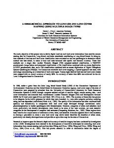
where P =probability that two adjacent pixels, randomly chosen, are of patch types ij i and j. Contagion will equal 100% when all patch types are equally adjacent to all other patch types, and approaches zero as the distribution of adjacencies becomes less even (McGarigal and Marks 1995). Contagion is sensitive to patch richness (Frohn 1998). 2.2.3. Fractal dimension from perimeter/area Fractal dimension calculated from perimeter/area has been used widely in landscape ecology to describe patch shape complexity. This index, based on the log-log regression of patch area to patch perimeter, does not give a true determination of fractal dimension because it is derived from measurements taken at only one scale (Frohn 1998). This index ranges from one to two; values close to one indicate a landscape made up of shapes with simple perimeters, and values close to two represent landscapes with very complex perimeters (McGarigal and Marks 1995). 3. Case study The objective of this study was to compare the performances of selected spatial statistics and landscape metrics to characterise diVerent land covers using unclassi ed Landsat Thematic Mapper (TM) data for a site in north-eastern Costa Rica. The purpose was to determine whether spatial landscape complexity can be captured by these methods, and whether these methods can be used to re ect the degree of human disturbance. The hypothesis was that complexity in a natural landscape decreases with increasing intensity of human activities. The methods evaluated were i) fractal dimension using the isarithm method, ii) fractal dimension using the modi ed TPSA method, iii) spatial autocorrelation, iv) Shannon’s diversity index, v) contagion, and vi) fractal dimension from perimeter/area. 3.1. Study area The study site is in the Caribbean lowlands of north-eastern Costa Rica (SarapiquÌ´ Canto´n, Province of Heredia), where the foothills of the Cordillera Volcanica Central meet the coastal plain ( gure 2). The site encompasses approximately 35 km by 40 km of lowland forests and agricultural lands that have undergone rapid change since the colonization of the frontier opened in the 1950s. This study is useful in a regional context because the proximate causes of change in the site are typical of
Spatial methods for characterising land cover for the tropics
2463
Figure 2. Study area, SarapiquÌ´ Canto´n, Costa Rica.
many lowland tropical areas, and include subsistence farming, small-scale commercial and plantation agriculture, cattle ranching, protected areas, and infrastructure development (Read et al. 2001). SarapiquÌ´ has gone from being an open frontier to one that contributes signi cantly to the Costa Rica’s agricultural export economy.
2464
J. M. Read and N. S-.N. L am
3.2. Data sources and preparation of subsets Unclassi ed georeferenced Landsat-TM data, acquired approximately 10 years apart, were used for these analyses; one scene from 1986, and two scenes from 1996 and 1997, both partially obscured by cloud cover. Rectangular or square areas representing a single cover type (closed forest, scrub, pasture, or agriculture) of approximately, and at least, 4096 pixels (333 hectares)1, were identi ed from the images based on land-cover maps generated from unsupervised classi cations (table 1) of the three Landsat-TM datasets (see Read et al. 2001 for details of classi cations). The classi cation scheme was designed to represent land-cover patterns in the site, speci cally for studying forest conversion rates, and patterns and trajectories of land-cover change. The four landcover classes included in the present study represent the most abundant cover types in the site, and also represent varying degrees of human disturbance. Subsets of the selected areas were generated of all seven Landsat-TM bands and the normalized diVerence vegetation index (NDVI). Where possible, subsets were selected from the same locations for the 1986 and 1996/1997 data for comparison (cloud cover in the 1996/1997 images prevented this in some cases). A total of 24 subsets were generated, representing ten forest, nine pasture, three agriculture, and two scrub areas ( gure 3). The subsets representing forest contained the most homogeneous cover of the four cover types because large extents of forest existed in both 1986 and 1996, and common areas for both dates could be selected. The pasture, agriculture and scrub classes had a more fragmented distribution across the landscape, thus, despite using unsupervised classi cations to aid subset selection, the cover within each subset was less homogeneous than the forest subsets, and common areas from both dates could not be isolated. 3.3. Analyses All analyses generated a single value for each band and NDVI dataset of each subset. Descriptive statistics were likewise extracted for each subset. Fractal dimensions using the isarithm and modi ed TPSA methods, and spatial autocorrelation, were calculated using the Image Characterization and Modelling System (ICAMS; Louisiana State University and National Aeronautics and Space Administration) (see Quattrochi Table 1.
Classi cation scheme.
Class
Description
Forest
Closed canopy forest; may include undisturbed old growth, selectively-logged, secondary. Young scrubby vegetation resulting from fallowed pastures and agricultural elds. Pastures used primarily for cattle. May include pastures with some degree of tree cover (mostly scattered individual trees, or groups of trees), although not closed canopy. Include annual and permanent crops; plantation agriculture. Urban ( buildings, roads); barren (i.e. river beaches). No data (mixed classes of clouds, cloud shadows, lakes, rivers).
Scrub Pasture Agriculture Other No data
1A minimum size of 26×26 (=4096) pixels was required for calculation of fractal dimension based on 6 steps. Each step represents a value in the regression equation used to determine D. See Lam et al. (1997) for details.
Spatial methods for characterising land cover for the tropics
Figure 3.
2465
1986 Landsat-TM image of the study area, showing an example subset for each cover type.
et al. 1997, Lam et al. 1998 for details). The TPSA method of calculating fractal dimension requires that the values be normalized for comparison, thus the subset values were stretched over 0–255 using a minimum/maximum stretch prior to running the TPSA algorithm. Both the TPSA and the isarithm algorithms were run using six steps, which provided six points for computing the linear regression. The isarithm algorithm was run using an interval of two. In ICAMS only D values from individual isarithms whose R2 values are 0.9 are included in the overall D calculation, and any isarithm for which a zero length is returned at any step size, is likewise rejected. Shannon’s diversity index, contagion, and fractal dimension from perimeter/area were computed for each subset using the FRAGSTATS spatial pattern analysis program (Oregon State University, Corvallis, OR). In addition, patch richness (i.e. the number of distinct pixel values or ‘patch types’) was calculated for each subset as a non-spatial measure of complexity. 4. Results and discussion 4.1. Descriptive statistics The band statistics for each subset showed typical vegetation re ectances, with high near-infrared returns and lower returns in the visible bands, for all four cover
J. M. Read and N. S-.N. L am
2466
types ( gure 4). Variation, measured as standard deviations, revealed the forest to have the least absolute variation of pixel values centred on its mean, whereas the agriculture, pasture and scrub classes had progressively more variation. This result could partially be explained by diVerences in the degree of homogeneity of land cover of the individual subsets, which in turn is a result of diVerences in the degree of fragmentation of the four land-cover types (see Read et al. 2001). The mean coeYcients of variation revealed low relative variation for the forest class for all bands in comparison with the other cover types ( gure 5). The high coeYcients of variation relative to the other bands for the near- and mid-infrared bands (bands 4, 5 and 7) indicate variation within each cover type in plant biomass, and plant and soil moisture conditions. The low variation found for the thermal band (band 6) can be attributed to the lower spatial resolution of the band, the eVects of resampling
Figure 4.
Subset means and standard deviations by cover type.
Figure 5. Subset coeYcients of variation by cover type.
Spatial methods for characterising land cover for the tropics
2467
the 120 m pixels to 28.5 m, and the naturally small variation in temperature across the landscape (see also Lam 1990). All cover types had high NDVI values, as expected for a predominantly vegetated landscape. Forest had the highest NDVI value, followed by scrub, pasture, and then agriculture. Variation in NDVI would be expected to be lower than the variation in bands 3 and 4 due to the reduction of the eVects of topography conferred by the NDVI transformation. This was found to be true for all cover types. 4.2. Fractal dimensions and spatial autocorrelation The isarithm method revealed consistently higher dimensions (D) than the TPSA method for agriculture, pasture, and scrub. Values for forest, however, showed mixed results, with the TPSA method yielding higher D values in the visible bands and in the mid-infrared band 7. This diVerence in the behaviour of the isarithm method could be a result of the low degree of absolute variation (described by the standard deviation) of pixel values within the forest class for these bands. This would mean that any existing variation could potentially be under-sampled depending on the isarithm interval and the speci c isarithms used, thereby yielding no result or a low value. This argument is supported by the lack of results for band 6 for all cover types, which had a very smooth distribution. The TPSA method yielded distinct values of D across all six non-thermal bands for all cover types ( gure 6). D values across cover types showed no relation to the coeYcients of variation of spectral values for all bands, a nding that supports Lam’s (1990) conclusion that both non-spatial and spatial statistics are necessary to fully characterise the variation in remotely-sensed data. Forest had the highest overall D for all bands and NDVI, suggesting a greater spatial complexity, or lower clustering, of pixel values within the class. Scrub, pasture, and agriculture showed progressively lower D values across the six non-thermal bands. These results support ndings of previous studies (Krummel et al. 1987, De Cola 1989) that showed decreasing values of D to be associated with cover types representing increasing degrees of human in uence. The large patches of relatively homogeneous banana plantations for example, yielded lower D values for all bands
Figure 6.
Fractal dimensions (triangular prism surface area method) by cover type.
2468
J. M. Read and N. S-.N. L am
and NDVI than the highly variable complex canopy structure of old-growth forests. Likewise, the scrub category, which is an intermediate category between forest and pasture, had a D value intermediate between the forest and pasture categories. Standard error plots for the isarithm and TPSA methods showed forest to have the smallest standard errors across all bands, and no overlap with other cover types ( gure 7). Agriculture, pasture, and scrub had overlapping standard errors, with agriculture consistently showing the greatest error across all bands. The large standard errors re ect the small sample size for agriculture (three subsets) and variation in D across the subsets. The subsets for agriculture, scrub and pasture were not as homogeneous as the forest subsets, and inclusion of some areas of the other two cover types were unavoidable, thus the overlap in standard errors of the means of these cover types would be expected. These results highlight the problem with ensuring an adequate number of points (steps) for calculating the regression on the one hand, and analysing areas that are too large to represent meaningful patterns on the landscape on the other. However, the cover types of scrub, pasture, and agriculture exist, by their nature, as smaller patches interspersed with each other, thus the subsets were valid representations of the complexity of these cover types. In order to extract D values for more homogeneous areas of these more fragmented cover types, ner spatial resolution data would be required. Calculation of D using Landsat-TM data however, does have potential for distinguishing forest from nonforest cover over large areas, such as the Amazon. De Jong and Burrough (1995) proposed a local TPSA method, whereby an image of D values is generated using moving windows. Such a procedure could be used in rapid change detection over large areas. Moran’s I index of spatial autocorrelation showed the forest to have low positive values for the non-thermal bands, in contrast to the other cover types ( gure 8). This suggests that the spatial distribution of pixel values for forest approached that of a random distribution rather than a clustered distribution. The pasture, agriculture and scrub showed higher index values, suggesting more clustered distributions of pixel values. The standard errors for Moran’s I showed scrub and agriculture to have consistently larger errors across bands than the forest and pasture classes, and
Figure 7.
Mean±1 standard error for fractal dimension (triangular prism surface area method) by cover type for band 3 ( band 3 shown as an example).
Spatial methods for characterising land cover for the tropics
2469
Figure 8. Spatial autocorrelation (Moran’s I) by cover type.
showed the mean value for forest to be distinct from the other cover types. Moran’s I and fractal dimension (TPSA) were inversely related. This result was expected because fractal dimension is low for clustered distributions and high for more fragmented distributions. 4.3. L andscape indices Patch richness (i.e. the number of distinct pixel values or ‘patch types’ in each subset) gives some indication of the variability of pixel values within each cover type. Forest was found to have the lowest number of pixel classes for all bands, with agriculture, pasture, and scrub showing progressively more classes. These results are comparable to the standard deviations (i.e. absolute variation) of pixel values about the mean. The forest had lower values of Shannon’s diversity index, S, than the other classes; scrub and pasture had high S values and agriculture intermediate values ( gure 9). Exceptions were band 4 and NDVI, which showed diVerent relative values across cover types. Contagion showed a less clear pattern than Shannon’s diversity index with landcover type ( gure 9). Generally, agriculture and forest showed relatively clumped distributions compared with the other cover types, and pasture and scrub showed less clumped/more interspersed distributions of pixel values. The forest had low values of contagion, however, for the vegetation-sensitive bands 4 and 5. Contagion values for NDVI showed no resemblance to the band responses. Approximately inverse relationships were demonstrated between contagion and patch richness (presumably a consequence of the sensitivity of the contagion metric to patch richness), and contagion and Shannon’s diversity index. The sensitivity of contagion and Shannon’s diversity index to patch richness was probably exaggerated in this study due to the high number of diVerent patch types (i.e. unclassi ed pixel values). As a result, these indices may not prove useful in characterising unclassi ed remotely-sensed data. The fractal dimension from perimeter/area yielded no clear patterns across cover types, but generally showed agriculture and pasture to have the lowest dimensions,
2470
J. M. Read and N. S-.N. L am
Figure 9. Selected landscape metrics by cover type.
Spatial methods for characterising land cover for the tropics Table 2.
Cover type Forest Scrub Pasture Agriculture
2471
Comparison of performances of selected methods.
Fractal Fractal Shannon’s dimension dimension Moran’s I Diversity (TPSA) (isarithm) Index Index * * * *
* * *
* * * *
Fractal dimension Contagion (perimeter/area) * * * *
* * * *
Gradient from dark to light shades represents high to low values across all bands and NDVI; *=no discernible pattern across all bands and NDVI.
and forest and scrub to have higher dimensions ( gure 9). DiVerences between classes became less clear for the vegetation-sensitive bands 4 and 5. The results of the landscape metrics would suggest that these metrics, as indicators of complexity for unclassi ed remotely-sensed data, do not provide additional information to those provided by fractal dimension, spatial autocorrelation, and standard band statistics (table 2). A possible explanation for this is that the landscape metrics do not make use of the absolute values of pixel DNs, nor the diVerences between pixel values, but simply recognize that they are diVerent from one another (i.e. diVerent patch types). Thus, the landscape metrics use less information than the spatial statistics, which make use of both the value and spatial arrangement of the pixel. 5. Conclusions This study explored the potential of selected methods for characterising land cover from Landsat-TM data for a lowland tropical environment, including two spatial statistics, and selected landscape pattern metrics. The results revealed that the fractal dimension, calculated using the TPSA method, and spatial autocorrelation were useful for distinguishing diVering degrees of spatial complexity represented by land-cover types. Speci cally, the ability of fractal signatures to distinguish forest and non-forest cover types in the study area was demonstrated. At the same time the transition from a high degree to a lower degree of human disturbance was revealed clearly by these two spatial statistics; from low D and high I for agriculture, to higher D and lower I for forest. The isarithm method of calculating fractal dimension was found to be sensitive to the degree of absolute spectral variation in a scene, and thus less robust than the TPSA method. Standard landscape metrics for measuring complexity in unclassi ed Landsat-TM data were not found to be useful due to the high number of ‘patch types’ inherent in the data, and the reduction in information when pixel values are considered only as distinct patch types. Our results demonstrate the inherent diVerences between geospatial statistics and landscape pattern metrics for describing land cover from unclassi ed remotely-sensed data, and highlight the potential of geospatial statistics for describing characteristics of the data that are not isolated by landscape pattern metrics. The potential of spatial statistics to characterise land cover and detect changes in land cover represents a new area of research that should be addressed. Calculation of fractal dimension and Moran’s I (and potentially other spatial statistics) could provide a rapid, automated technique for identi cation of hot spots of change (for instance, tropical deforestation) from data derived from diVerent sensors and at
2472
J. M. Read and N. S-.N. L am
diVerent scales. These methods also have potential for analysis of large (regional or global) areas because processing times are rapid. In addition, these two spatial statistics could serve to improve land-cover classi cations in areas where cover types with contrasting degrees of anthropogenic in uence exist, such as in forest environments undergoing diVerent management regimes. The results of this research suggest several avenues for further studies. First, the eVects of seasonality on fractal dimension and spatial autocorrelation should be investigated. This study was conducted for a lowland tropical site that does not exhibit marked seasonality and we expect that results from diVerent times of year would be comparable. However, in temperate regions, where seasonality is stronger, we expect that the results will vary with changes in phenology and snow cover (see Quattrochi et al. 2001). Another potential area of research is to assess these methods using image transformations other than NDVI, such as Principal Components and Tasselled Cap transformations. Finally, the emphasis of this study was to assess landscape complexity based on the degree of human disturbance. The analyses could be extended to assess complexity due to other factors, such as topography, hydrology, phenology, and geology. Acknowledgments Funding for this research was provided by the U.S. National Science Foundation (grant SBR-9627957), Space Imaging EOSAT Co., and a Robert C. West Award (Department of Geography and Anthropology, Louisiana State University). The authors are grateful for logistic support provided by the Organization for Tropical Studies and La Selva Biological Station in Costa Rica, and by the Department of Geography and Anthropology at Louisiana State University. The authors thank two anonymous reviewers for their helpful comments. References Brodley, C. E., Lane, T., and Stough, T. M., 1999, Knowledge discovery and data mining. American Scientist, 87, 54–61. Chuvieco, E., 1999, Measuring changes in landscape pattern from satellite images: short-term eVects of re on spatial diversity. International Journal of Remote Sensing, 20, 2331–2346. Cihlar, J., 2000, Land cover mapping of large areas from satellites: status and research priorities. International Journal of Remote Sensing, 21, 1093–1114. Clarke, K. C., 1986, Computation of the fractal dimension of topographic surfaces using the triangular prism surface area method. Computers and Geosciences, 12, 713–722. Cliff, A. D., and Ord, J. K., 1973, Spatial Autocorrelation (London: Pion). De Cola, L., 1989, Fractal analysis of a classi ed Landsat scene. Photogrammetric Engineering and Remote Sensing, 55, 601–610. de Jong, S. M., and Burrough, P. A., 1995, A fractal approach to the classi cation of Mediterranean vegetation types in remotely sensed images. Photogrammetric Engineering and Remote Sensing, 61, 1041–1053. Emerson, C. W., Lam, N. S.-N., and Quattrochi, D. A., 1999, Multi-scale fractal analysis of image texture and pattern. Photogrammetric Engineering and Remote Sensing, 65, 51–61. Fayyad, U., Haussler, D., and Stolorz, P., 1996, Mining scienti c data. Communications of the ACM, 39, 51–57. Franklin, S. E., Hall, R. J., Moskal, L. M., Maudie, A. J., and Lavigne, M. B., 2000, Incorporating texture into classi cation of forest species composition from airborne multispectral images. International Journal of Remote Sensing, 21, 61–79. Friedl, M. A., and Brodley, C. E., 1997, Decision tree classi cation of land cover from remotely sensed data. Remote Sensing of Environment, 61, 399–409.
Spatial methods for characterising land cover for the tropics
2473
Friedl, M. A., Brodley, C. E., and Strahler, A. H., 1999, Maximizing land cover classi cation accuracies produced by decision trees at continental to global scales. IEEE T ransactions on Geoscience and Remote Sensing, 37, 969–977. Frohn, R. C., 1998, Remote Sensing for L andscape Ecology: New Metric Indicators for Monitoring, Modeling, and Assessment of Ecosystems (Boca Raton, FL: Lewis Publishers, CRC Press). Griffiths, J. L., Lee, J., and Eversham, B. C., 2000, Landscape pattern and species richness; regional scale analysis from remote sensing. International Journal of Remote Sensing, 21, 2685–2704. Houghton, R. A., 1994, The worldwide extent of land-use change. BioScience, 44, 305–313. Jaggi, S., Quattrochi, D. A., and Lam, N. S.-N., 1993, Implementation and operation of three fractal measurement algorithms for analysis of remote-sensing data. Computers and Geosciences, 19, 745–767. Klinkenberg, B., and Goodchild, M. F., 1992, The fractal properties of topography: a comparison of methods. Earth Surface Processes and L andforms, 17, 217–234. Krummel, J. R., Gardner, R. H., Sugihara, G., O’Neill, R. V., and Coleman, P. R., 1987, Landscape patterns in a disturbed environment. Oikos, 48, 321–324. Lam, N. S.-N., 1990, Description and measurement of Landsat TM images using fractals. Photogrammetric Engineering and Remote Sensing, 56, 187–195. Lam, N. S.-N., and De Cola, L. (Eds.), 1993a, Fractals in Geography (Englewood CliVs, New Jersey: Prentice Hall). Lam, N. S.-N., and De Cola, L., 1993b, Fractal Measurement. In Fractals in Geography, Eds. Lam, N. S.-N., and De Cola, L. (Englewood CliVs, New Jersey: Prentice Hall), pp. 23–55. Lam, N. S.-N., and Qiu, H.-L., 1992, The fractal nature of the Louisiana coastline. In Geographical Snapshots of North America, Ed. Janelle, D. G. (New York: The Guilford Press), pp. 270–274. Lam, N. S.-N., Qiu, H.-L,. and Quattrochi, D., 1997, An evaluation of fractal surface measurement methods using ICAMS (Image Characterization and Modeling System). ACSM/ASPRS Annual Convention, Vol. 5 (Seattle, WA: ASPRS and ACSM), pp. 377–386. Lam, N. S.-N., Quattrochi, D., Qiu, H.-L., and Zhao, W., 1998, Environmental assessment and monitoring with image characterization and modeling system using multiscale remote sensing data. Applied Geographic Studies, 2, 77–93. Lam, N. S.-N., and Quattrochi, D. A., 1992, On the issues of scale, resolution, and fractal analysis in the mapping sciences. Professional Geographer, 44, 88–98. Lambin, E. F., 1997, Modelling and monitoring land-cover change processes in tropical regions. Progress in Physical Geography, 21, 375–393. Li, H., and Reynolds, J. F., 1993, A new contagion index to quantify spatial patterns of landscapes. L andscape Ecology, 8, 155–162. Li, H., and Reynolds, J. F., 1994, A simulation experiment to quantify spatial heterogeneity in categorical maps. Ecology, 75, 2446–2455. Lillesand, T. M., and Kiefer, R. W., 2000, Remote Sensing and Image Interpretation, 4th edn (New York: John Wiley & Sons, Inc). Mandlebrot, B., 1967, How long is the coast of Britain? Statistical self-similarity and fractional dimension. Science, 156, 636–638. Mas, J.-F., 1999, Monitoring land-cover changes: a comparison of change detection techniques. International Journal of Remote Sensing, 20, 139–152. McGarigal, K., and Marks, B. J., 1995, FRAGSTATS: spatial pattern analysis program for quantifying landscape structure (Portland, OR: U.S. Department of Agriculture, Forest Service, Paci c Northwest Research Station), pp. 122. McGuffie, K., Henderson-Sellers, A., Zhang, H., Durbidge, T. B., and Pitman, A. J., 1995, Global climate sensitivity to tropical deforestation. Global and Planetary Change, 10, 97–128. Myers, N., 1993, Tropical forests: the main deforestation fronts. Environmental Conservation, 20, 9–16. Nunes, C., and Auge, J. I. (Eds.), 1999, L and-Use and L and-Cover Implementation Strategy (Stockholm: IGBP).
2474
Spatial methods for characterising land cover for the tropics
Palubinskas, G., Lucas, R. M., Foody, G. M., and Curran, P. J., 1995, An evaluation of fuzzy and texture-based classi cation approaches for mapping regenerating tropical forest classes from Landsat-TM data. International Journal of Remote Sensing, 16, 747–759. Peralta, P., and Mather, P., 2000, An analysis of deforestation patterns in the extractive reserves of Acre, Amazonia from satellite imagery: a landscape ecological approach. International Journal of Remote Sensing, 21, 2555–2570. Qiu, H.-L., Lam, N. S.-N., Quattrochi, D. A., and Gamon, J. A., 1999, Fractal characterization of hyperspectral imagery. Photogrammetric Engineering and Remote Sensing, 65, 63–71. Quattrochi, D. A., Emerson, C. W., Lam, N. S.-N., and Qiu, H.-L., 2001, Fractal characterization of multitemporal remote sensing data. In Modelling Scale in Geographical Information Science, Eds. Tate, N., and Atkinson, P. (West Sussex, England: John Wiley & Sons, Ltd), pp. 13–34. Quattrochi, D. A., Lam, N. S.-N., Qiu, H.-L., and Zhao, W., 1997, Image Characterization and Modeling System (ICAMS): A geographic information system for the characterization and modeling of multi-scale remote sensing data. In Scale in Remote Sensing and GIS, Eds. Quattrochi, D. A., and Goodchild, M. F. (Boca Raton, FL: CRC Lewis Publishers), pp. 295–307. Read, J. M., Denslow, J. S., and Guzman, S. M., 2001, Documenting land-cover history of a humid tropical environment in northeastern Costa Rica using time-series remotely sensed data. In Remote Sensing and GIS in Biogeography and Ecology, Eds. Millington, A. C., Walsh, S. D., and Osborne, P. E. (Boston: Kluwer), pp. 69–89. Rees, W. G., 1992, Measurement of the fractal dimension of ice-sheet surfaces using Landsat data. International Journal of Remote Sensing, 13, 663–671. Seixas, J., 2000, Assessing heterogeneity from remote sensing images: the case of deserti cation in southern Portugal. International Journal of Remote Sensing, 21, 2645–2663. Singh, A., 1989, Digital change detection techniques using remotely-sensed data. International Journal of Remote Sensing, 10, 989–1003. Tucker, C. J., and Townshend, J. R. G., 2000, Strategies for monitoring tropical deforestation using satellite data. International Journal of Remote Sensing, 21, 1461–1471. Vitousek, P. M., 1992, Global environmental change: an introduction. Annual Review in Ecology and Systematics, 23, 1–14. Walker, B. H., and Steffen, W. L., 1996, GCTE science: objectives, structure and implementation. In Global Change and T errestrial Ecosystems, Eds. Walker, B., and SteVen, W. (Cambridge: Cambridge University Press), pp. 3–9. Xavier, B., and Szejwach, G. (Eds.), 1998, L UCC Data Requirements Workshop: survey of needs, gaps and priorities on data for land-use/land-cover change research (Barcelona, Spain: Institut Cartogra c de Catalunya). Zhan, X., Defries, R., Townshend, J. R. G., Dimiceli, C., Hansen, M., Huang, C., and Sohlberg, R., 2000, The 250 m global land cover change product from the Moderate Resolution Imaging Spectroradiometer of NASA’s Earth Observing System. International Journal of Remote Sensing, 21, 1433–1460.