tries known as spatial partitions that are able to model maps containing ... tions, spatial systems tend to represent space as collections of individual points,.
Spatial Partition Graphs: A Graph Theoretic Model of Maps Mark McKenney and Markus Schneider� University of Florida, Department of Computer and Information Sciences {mm7,mschneid}@cise.ufl.edu
Abstract. The notion of a map is a fundamental metaphor in spatial disciplines. However, there currently exist no adequate data models for maps that define a precise spatial data type for map geometries for use in spatial systems. In this paper, we consider a subclass of map geometries known as spatial partitions that are able to model maps containing region features. However, spatial partitions are defined using concepts such as infinite point sets that cannot be directly represented in computers. We define a graph theoretic model of spatial partitions, called spatial partition graphs, based on discrete concepts that can be directly implemented in spatial systems.
1
Introduction
In spatially oriented disciplines such as geographic informations systems (GIS), spatial database systems, computer graphics, computational geometry, computer vision, and computer aided design, a map is a fundamental metaphor. Many of these systems fundamentally represent space through more primitive concepts, such as points, lines, or regions, which we denote the traditional spatial types. These more basic representations of space are often combined to form maps in many applications. Furthermore, in applications such as GIS, global positioning systems, and navigation systems, the map itself tends to play a central role in that the map is the primary user interface tool. Thus, users tend to manipulate data in terms of maps instead of the underlying types of point, line, and region. Despite the intimate ties between maps and a wide variety of spatial applications, spatial systems tend to represent space as collections of individual points, lines, and regions, and utilize maps as a visualization tool for these more simple types. For example, a system may display a collection of regions to a user as a map, but the system itself can only process space based on points, lines, and regions. Thus, a map in this sense is not being used as a representation of space, but as a visualization of more basic spatial entities. However, treating a map simply as a visualization gives rise to problems at both the conceptual and implementation levels. At the conceptual level, maps must conform to some set of properties in order to handle certain configurations of map components. �
This work was partially supported by the National Science Foundation under grant number NSF-CAREER-IIS-0347574.
D. Papadias, D. Zhang, and G. Kollios (Eds.): SSTD 2007, LNCS 4605, pp. 167–184, 2007. c Springer-Verlag Berlin Heidelberg 2007 �
168
M. McKenney and M. Schneider
Consider two regions r and s such that s fits completely in the interior of r. If a user attempts to construct a map visualization of these regions, then it is possible that s will be completely hidden by r, indicating that some set of properties is required to govern the construction of maps. Therefore, even when using maps only as visualizations, a type definition of maps is required that poses constraints on the map contents and indicates how situations such as this one should be handled. Furthermore, map operations are not purely geometric. For example, components of maps are typically labeled with thematic information (e.g., names of states, cities, rivers, etc.). When considering the intersection of two maps, not only must a spatial intersection operation be defined, but some method of labelling the resulting map must be defined too that takes into account the labels of the argument maps. At the implementation level, systems that utilize maps as visualization tools cannot take advantage of map properties in algorithms. For example, maps implicitly model topological relationships such as the adjacency between regions. Thus querying a map for neighborhoods of adjacent regions or regions that are disjoint from a query region is intuitive and simple in the map context. Given a spatial system that cannot take advantage of map properties, maps must be simulated as collections of other spatial objects and such topological information must be calculated explicitly. Additionally, when implementing operations such as map intersection in such systems, a Cartesian product of both collections of spatial objects must be computed. In this paper, we take the view that maps themselves are a spatial data type, and not merely a visualization tool. We view a map as a map geometry, i.e., as a spatial data type with its own type definition and operations. The idea of using map geometries to represent space in spatial systems aligns nicely with the current practice of having users interact with spatial systems through maps. As was mentioned before, maps implicitly model topological relationships between the spatial components, such as regions, within the map. Furthermore, the use of map geometries in spatial systems unifies the user interface model and the data model such that user queries can be computed over maps. Despite the advantages that processing space in map form provides for spatial systems, research into modeling maps has not resulted in an adequate data model for maps (see Section 2). Current models define maps as sets of traditional spatial types. These models lack a mechanism to enforce constraints over the traditional types, and tend to lack closure properties. Conceptual models exist that define abstract mathematical models of map geometries that are able to address problems other models have with constraint enforcement and closure concerns; however, such models rely on concepts such as infinite point sets and mappings that cannot be directly implemented in computer systems. In this paper, we only consider a particular subclass of map geometries that we call spatial partitions. A spatial partition is a subdivision of the plane into regions such that each region has a label that identifies it and its characteristic thematic properties, and regions either meet or are disjoint with one another. We do not consider map geometries that contain features such as line networks or spatial
Spatial Partition Graphs: A Graph Theoretic Model of Maps
169
point entities, but leave this to future work. By considering map geometries as spatial partitions, we are able to model a map as a single entity containing regional features satisfying particular topological constraints and define operations and predicates over it. We provide the formal definition of spatial partitions in Section 4. However, this definition is not sufficient for modeling map geometries in spatial systems because it defines an abstract model of spatial partitions. The main contribution of this paper is the unique characterization of a spatial partition as a spatially embedded graph called a spatial partition graph. We define the type of spatial partition graphs along with constraints for these graphs that are enforced implicitly by the data type. Furthermore, we define spatial partition graphs at the discrete level, meaning that the definition avoids concepts such as infinite point sets that cannot be directly represented in computers. The result is a precise conceptual data type for map geometries that can be directly implemented in computer systems. Thus, our model resolves the existing conceptual and implementation level problems associated with current uses of map visualizations in spatial systems. Because we define a graph theoretic model, it is possible to directly utilize the many known graph algorithms for implementing operations such as reachability and connectivity. Finally, a discrete definition of map geometries provides a foundation upon which new algorithms for map operations can be specified. In Section 2, we discuss related research into spatial data types for map geometries. The abstract model of spatial partitions, upon which we base our model of spatial partition graphs, is presented formally in Section 3. In Section 4, we define and discuss the properties of spatial partition graphs. Finally, in Section 5, we draw some conclusions.
2
Related Work
Research into spatial data types has focused on the development of simple and complex points, lines, and regions. Simple lines are continuous, one-dimensional features embedded in the plane with two endpoints; simple regions are two dimensional point sets that are topologically equivalent to a closed disc. Increased application requirements and a lack of closure properties of the simple spatial types lead to the development of the complex spatial types. In [1], the authors formally define complex data types, such as complex points (a single point object consisting of a collection of simple points), complex lines (which can represent networks such as river systems), and complex regions that are made up of multiple faces and holes (i.e., a region representing Italy, its islands, and the hole representing the Vatican). These types are defined based on concepts from point set topology, which allow the identification of the interior, exterior, and boundary of spatial the types. The notations S ◦ , ∂S, and S − respectively indicate the interior, boundary, and exterior of a point, line, or region spatial data type. The idea of a map as a spatial data type has received significant attention in the literature. In [2,3,4,5], a map is not defined as a data type itself, but as a collection of spatial regions that satisfy some topological constraints.
170
M. McKenney and M. Schneider
Because these map types are essentially collections of more basic spatial types, it is unclear how the topological constraints can be enforced, and how thematic information can be effectively modeled. Furthermore, these models focus on an implementation model that can be directly incorporated into spatial systems while neglecting spatial data type considerations such as closure of maps under map operations. Other approaches [6,7] to defining map types have focused on raster or tessellation models. However, such approaches are not general enough for our purposes in the sense that the geometries of maps in these models are restricted to the tessellation scheme in use. In [8], the authors consider a map to be a planar subdivision; however, they do not discuss how a planar subdivision should be modeled except to say that data structures such as winged edge or quad edge structures should be used. The work that comes closest to ours is [9,10] in which the authors consider modeling maps as special types of plane graphs. However, the authors of these works define such graphs based on modeling a map as a collection type consisting of spatial point, line, and region objects. Problems in the proposed methods arise when different spatial objects in the map share coordinates. For example, given the method of deriving a plane graph from a collection of points, lines, and regions, it is unclear if a spatial point object that has the same coordinates as the endpoint of a spatial line object in the plane graph can be distinguished. Furthermore, the authors require a separate structure to model what they term the combinatorial structure of a plane graph, which includes the topological relationships between different spatial components of the graph. Finally, the plane graph, as defined, is not able to model thematic properties of the map. We base our work on the model of maps presented in [11]. The authors of this paper define an abstract, mathematical data model that formally describes the type of spatial partitions. A spatial partition is the partitioning of the plane into regular, open point sets such that each point set is associated with a label. The use of labels to identify point sets allows thematic information to be modeled explicitly in spatial partitions. Furthermore, operations are defined over spatial partitions, and it is shown that the operations are closed over the type of spatial partitions. A detailed description of the type of spatial partitions is provided in Section 3. The main drawback to this model is that it is based on the concepts of infinite point sets and mappings that are not able to be represented discretely.
3
The Spatial Partition Model
In this section, we review the definition of spatial partitions upon which we base our graph model of spatial partitions. We begin by providing a high level description of the type of spatial partitions that indicates their properties and introduces their terminology. We then introduce the mathematical notation and definitions required to formally define spatial partitions. Finally, the formal mathematical type definition of spatial partitions is presented.
Spatial Partition Graphs: A Graph Theoretic Model of Maps
3.1
171
Description of Spatial Partitions
A spatial partition, in two dimensions, is a subdivision of the plane into pairwise disjoint regions such that each region is associated with a label or attribute having simple or complex structure, and these regions are separated from each other by boundaries. The label of a region describes the thematic data associated with the region. All points within the spatial partition that have an identical label are part of the same region. Topological relationships are implicitly modeled among the regions in a spatial partition. For instance, neglecting common boundaries, the regions of a partition are always disjoint; this property causes maps to have a rather simple structure. Note that the exterior of a spatial partition (i.e., the unbounded face) is always labeled with the ⊥ symbol. Figure 1a depicts an example spatial partition consisting of two regions. We stated above that each region in a spatial partition is associated with a single attribute or label. A spatial partition is modeled by mapping Euclidean space to such labels. Labels themselves are modeled as sets of attributes. The regions of the spatial partition are then defined as consisting of all points which contain an identical label. Adjacent regions each have different labels in their interior, but their common boundary is assigned the label containing the labels of both adjacent regions. Figure 1b shows an example spatial partition complete with boundary labels. In [11], operations over spatial partitions are defined based on known map operations in the literature. It is shown that all known operations over spatial partitions can be expressed in terms of three fundamental operations: intersection, relabel, and refine. Furthermore, the type of spatial partitions is shown to be closed under these operations, indicating that the type of spatial partitions is closed under all known operations over them. In this paper, we only require the use of the refine operation, which is discussed later. We direct the reader to [11] for the definitions of intersection and relabel due to space constraints. {A, {A}
{A}
} {A}
{A}
{ }
{ } {A,B}
{B}
{A,
}
{B}
{A, {B,
{ }
a
}
} {A,B,
}
{ }
b
Fig. 1. Figure a shows a spatial partition with two regions and annotated with region labels. Figure b shows the same spatial partition with its region and boundary labels. Note that labels are modeled as sets of attributes in spatial partitions.
3.2
Notation
We now briefly summarize the mathematical notation used throughout the following sections. The application of a function f : A → B to a set of values
172
M. McKenney and M. Schneider
S ⊆ A is defined as f (S) := {f (x)|x ∈ S} ⊆ B. In some cases we know that f (S) returns a singleton set, in which case we write f [S] to denote the single element, i.e. f (S) = {y} =⇒ f [S] = y. The inverse function f −1 : B → 2A of f is defined as f −1 (y) := {x ∈ A|f (x) = y}. It is important to note that f −1 is a total function and that f −1 applied to a set yields a set of sets. We define the range function of a function f : A → B that returns the set of all elements that f returns for an input set A as rng(f ) := f (A). Let (X, T ) be a topological space [12] with topology T ⊆ 2x , and let S ⊆ X. The interior of S, denoted by S ◦ , is defined as the union of all open sets that are contained in S. The closure of S, denoted by S is defined as the intersection of all closed sets that contain S. The exterior of S is given by S − := (X − S)◦ , and the boundary or frontier of S is defined as ∂S := S ∩ X − S. An open set is ◦ regular if A = A [13]. In this paper, we deal with the topological space R2 . A partition of a set S, in set theory, is a complete decomposition of the set S into � non-empty, disjoint subsets {Si |i ∈ I}, called blocks: (i) ∀i ∈ I : Si = ∅, (ii) i∈I Si = S, and (iii) ∀i, j ∈ I, i = j : Si ∩ Sj = ∅, where I is an index set used to name different blocks. A partition can equivalently be regarded as a total and surjective function f : S → I. However, a spatial partition cannot be defined simply as a set-theoretic partition of the plane, that is, as a partition of R2 or as a function f : R2 → I, for two reasons: first, f cannot be assumed to be total in general, and second, f cannot be uniquely defined on the borders between adjacent subsets of R2 . 3.3
The Definition of Spatial Partitions
In [11], spatial partitions have been defined in several steps. First a spatial mapping of type A is a total function π : R2 → 2A . The existence of an undefined element ⊥A is required to represent undefined labels (i.e., the exterior of a partition). Definition 1 identifies the different components of a partition within a spatial mapping. The labels on the borders of regions are modeled using the power set 2A ; a border of π (Definition 1(ii)) is a block that is mapped to a subset of A containing two or more elements, as opposed to a region of π (Definition 1(i)) which is a block mapped to a singleton set. The interior of π (Definition 1(iii)) is defined as the union of π’s regions. The boundary of π (Definition 1(iv)) is defined as the union of π’s borders. The exterior of π (Definition 1(v)) is the block mapped ⊥A . As an example, let π be the spatial partition in Figure 1 of type X = {A, B, ⊥}. In this case, rng(π) = {{A}, {B}, {⊥}, {A, B}, {A, ⊥}, {B, ⊥}, {A, B, ⊥}}. Therefore, the regions of π are the blocks labeled {A}, {B}, and {⊥} and the boundaries are the blocks labeled {A, B}, {A, ⊥}, {B, ⊥}, and {A, B, ⊥}. Figure 2 provides a pictorial example of the interior, exterior, and boundary of a more complex example map (note that the borders and boundary consist of the same points, but the boundary is a single point set whereas the borders are a set of point sets).
Spatial Partition Graphs: A Graph Theoretic Model of Maps
a
b
c
173
d
Fig. 2. Figure a shows a spatial partition π with two disconnected faces, one containing a hole. The interior (π ◦ ), boundary (∂π), and exterior (π − ) of the partition are shown if Figures b c, and d, respectively. Note that the labels have been omitted in order to emphasize the components of the spatial partition.
Definition 1. Let π be a spatial mapping of type A (i) ρ(π) := π −1 (rng(π) ∩ {X ∈ 2A | |X| = 1}) −1 A (ii) ω(π) := � π (rng(π) ∩ {X ∈ 2 | |X| > 1}) (iii) π ◦ := r∈ρ(π)|π[r]�=⊥A r � (iv) ∂π := b∈ω(π) b (v) π − := π −1 ({⊥A })
(regions) (borders) (interior ) (boundary) (exterior )
A spatial partition of type A is then defined as a spatial mapping of type A whose regions are regular open sets [13] and whose borders are labeled with the union of labels of all adjacent regions. From this point forward, we use the term partition to refer to a spatial partition. Definition 2. A spatial partition of type A is a spatial mapping π of type A with: (i) ∀r ∈ ρ(π) : r = r ◦ (ii) ∀b ∈ ω(π) : π[b] = {π[r]|r ∈ ρ(π) ∧ b ⊆ ∂r} As was mentioned before, the type of spatial partitions is closed under all known partition operations. In this paper, we require the use of the refine operation. We provide a high-level description of the operation, and direct the reader to [11] for the formal definition. The refine operation uniquely identifies the connected components of a partition. Recall that two regions in a partition can share the same label if they are disjoint or meet at a point. Given a partition π containing multiple regions with the same label, the operation refine(π) returns a partition with identical structure to π, but with every region having a unique label. This is achieved by appending an integer to the label of each region that shares a label with another region. Figure 3 shows an example partition and the same partition after performing a refine operation. Note that the notation (A, 1) indicates that the integer 1 has been appended to label A. The boundary of a spatial partition implicitly imposes a graph on the plane. Specifically, the boundaries form an undirected planar graph. The edges of the graph are the points mapped to the boundaries between two regions. The vertices of the graph are the points mapped to boundaries between three or more regions. We identify edges and vertices based on the cardinality of their labels. However, due to degenerate cases, we must use the refinement of a partition to identify
174
M. McKenney and M. Schneider { }
{ }
{C, } {A} {A} {A, }
{A,C}
{C}
{C, }
{A,C} {A, }
a
{C, } {(A,1)} {(A,1),C} {C} {(A,1), }
{C, }
{(A,2),C} {(A,2)} {(A,2), }
b
Fig. 3. Figure a shows a spatial partition with two regions and its boundary and region labels. Figure b shows the result of the refine operation on Figure a.
these features. We define the set of edges and vertices imposed on the plane by a spatial partition as follows: Definition 3. Boundary points of a spatial partition π are classified as being a vertex or as being part of an edge by examining the refinement σ = refine(π) as follows: (i) �(π) = {b ∈ ω : |σ(b)| = 2} (ii) ν(π) = {b ∈ ω : |σ(b)| > 2}
4
A Discrete Model of Maps
The abstract model of spatial partitions maps each point in the plane to a specific label. However, computers provide only a finite resolution for the representation of data which is not adequate for the explicit representation of abstract spatial partitions. In order to represent maps in computers, a discrete map model is required that preserves the properties of spatial partitions while providing a representation that is suitable for storage and manipulation in computers. In this section, we provide a graph model of spatial partitions, which is a graph theoretic, discrete model of spatial partitions. Note that there is some ambiguity among graph terms in the literature, especially concerning terms indicating graphs that are allowed to contain loops and multiple edges between pairs of vertices. We begin this section by first providing an overview of graph terms and definitions that we use to develop our model. 4.1
Definitions from Graph Theory
In graph theory, a graph is a pair G = (V, E) of disjoint sets such that V is a set of vertices and E ⊆ V × V is a set of vertex pairs indicating edges between vertices. We denote the sets of vertices and edges for a given graph g as V (g) and E(g), respectively. A multigraph is a pair GM = (V, E) of disjoint sets with a mapping E → V × V allowing a multigraph to have multiple edges between a given pair of vertices. A loop in a graph is an edge that has a single vertex as both of its endpoints. A multigraph with loops is a pseudograph, and is defined as a pair GP = (V, E) with a mapping E → V × V . Finally, a nodeless pseudograph is a pseudograph that (possibly) contains edges that form loops that connect no vertices and that intersect no other edges or vertices. We define a nodeless pseudograph as a triple GN = (V, E, N ) (where N is the set of nodeless edges) with mapping E → V × V .
Spatial Partition Graphs: A Graph Theoretic Model of Maps
175
A path is a non-empty graph P = (V, E) such that V = {v1 , . . . , vn }, E = {v1 v2 , . . . , vn−1 vn } and all vi are distinct. Given a graph g = (V, E), a path of g is a graph p = (Vp , Ep ) where Vp ⊆ V (g) ∧ Ep ⊆ E(g) where p satisfies the definition of a path. A cycle is a path whose first and last vertices are identical, defined by a non-empty graph C = (V, E) such that V = {v1 , . . . , vn }, E = {v1 v2 , . . . , vn v1 } where all vi are distinct and n ≥ 3. Given a graph g = (V, E), a cycle of g is a graph c = (Vc , Ec ) where Vc ⊆ V (g) ∧ Ec ⊆ E(G) where c satisfies the definition of a cycle. The length of a cycle is the number of its edges. A polygonal arc is the union of finitely many straight line segments embedded into the plane and is homeomorphic to the closed unit interval [0, 1]. We use the terms arc and polygonal arc interchangeably. A graph is planar if it can be embedded in the plane such that no two edges intersect. A particular drawing of a graph is an embedding of the graph. A particular planar graph can have multiple embeddings in the plane such that edges in each embedding are drawn differently. A particular embedding of a planar graph is a plane graph. Formally, a plane graph is a pair (V, E) such that V ⊆ R2 , every edge is an arc between two vertices, the interior of an edge contains no vertex, and no two edges intersect except at their vertices. A plane graph g may contain cycles. We say a cycle c in plane graph g is minimal if there does not exist a path in g that splits the polygon induced by c into two pieces. We use the notation C(g) to indicate the set of minimal cycles in the graph g. 4.2
Representing Spatial Partitions as Graphs
In this section, we define the type of spatial partition graphs that is able to model both the structural and labelling properties of spatial partitions in a graph. We first attempt to define a graph based on the vertex and edge structure of a partition, but show that this is not sufficient because the labels of the partition are not explicitly represented in such a graph. We then define a new type of graph that is capable of representing both the structural and labelling properties of a spatial partition and that is defined based on discrete concepts. We then show how such a graph can be obtained from a given spatial partition. Recall that in the abstract model of spatial partitions, we can identify a graph structure based on the boundary of a partition π. Specifically, we observe that we can identify ν(π), the set of points that are vertices, and �(π), the set of point sets belonging to edges of a partition. However, we cannot simply assign the vertices and edges to a pair (V, E) in order to achieve a graph representation of π since it is possible for nodeless edges to be present in �(π). For example, the boundary of the rightmost face of region A in Figure 1 is composed of two nodeless edges; these edges are nodeless because the label of every point they contain is a set containing two attributes (i.e., no point in the edge satisfies the definition of a vertex in a partition). Therefore, we must use a triple (V, E, N ) consisting of the sets of vertices, edges, and nodeless edges to represent a partition as a graph. Deriving the set V from a partition π is trivial because we can directly identify the set of vertex points ν(π). Definition 3 defines the set of all edges of π as �(π); thus, it does not differentiate between edges and nodeless edges. It follows that
176
M. McKenney and M. Schneider
{(A,1),
}
{(A,2)}
{(A,1)} { } {(A,1),B}
{(A,2),
{B}
} {(A,2),
{B,
}
} {(A,1),B,
}
{ }
a
b
Fig. 4. Figure a shows the refinement of the partition in Figure 1a. Figure b shows the SSPG of a. Nodeless edges are dashed.
the set of nodeless edges of a partition, N , is a subset of �(π), but we cannot identify N by simply examining labels. Intuitively, the label of a nodeless edge should not form a subset of the label of any vertex. However, in Figure 1, the label of the boundary of the upper border of the left face of region A and the labels of both borders of the right face of region A are the same. Therefore, we cannot necessarily differentiate nodeless edges from edges by comparing labels. We can circumvent this problem if we can differentiate identically labeled edges from different faces of the same region. This can be achieved through the refine operation. Each nodeless edge in π can be identified as an edge in σ = refine(π) whose label does not form a subset of any vertex label (a vertex lies on an edge in the refinement of a partition iff the edge label is a subset of the vertex label). Note that the refine operation does not alter the edge structure of a partition, only its labels. Therefore, we can use σ = refine(π) to identify the set of nodeless edges N in π by saying that each edge in σ whose label does not form a subset of any vertex label in σ is in the set N . The edges of π can then be calculated as E = �(π)−N . Figure 4a shows the refinement of the partition in Figure 1. Figure 4b shows the graph representation of the partition in Figure 4a obtained by the method described above (nodeless edges are dashed). Because deriving a graph from a partition in this fashion results in a graph that exactly represents the edge structure of the partition from which it is derived, we call this type of graph a structural spatial partition graph (SSPG), and define it formally as follows: Definition 4. Given a spatial partition π of type A and its refinement σ = refine(π), we construct a structural spatial partition graph SSP G = (V, E, N ) with: V = ν(π) E = �(σ) − N N = {n ∈ �(σ)|�v ∈ ν(σ) : σ(n) ⊆ σ(v)} The SSPG is able to represent the structural aspects of a spatial partition, but it does not maintain the labelling information of the partition. Because a SSPG is defined based on a given partition, the spatial mapping for the partition is known. Therefore, the label for any edge or vertex in a SSPG can be determined through the associated spatial mapping, but this is insufficient for our purposes as we require an explicit representation of labels. However, the SSPG has the property that it is a plane nodeless pseudograph (PNP):
Spatial Partition Graphs: A Graph Theoretic Model of Maps
177
Theorem 1. Given a partition π of type A, its corresponding SSPG is a plane nodeless pseudograph. Proof. The definition of a nodeless graph states that a nodeless graph may contain nodeless edges; therefore, an SSPG is nodeless by definition. Similarly, the definition of a pseudograph states that the graph may contain multiple edges between the same vertices and loops. An SSPG is therefore a pseudograph by definition because it does not exclude such features. Now we must prove that a SSPG is a plane graph. The edges of an SSPG are taken directly from a spatial partition, which is embedded in R2 , indicating that the SSPG is an embedded graph. By the definition of spatial partitions, an edge in a partition is a border defined by a one-dimensional point set consisting of points mapped to a single label. Furthermore, this label is derived from the regions which the border separates. Assume that there exists two borders in a spatial partition that cross, which implies that the SSPG for this partition will contain two edges that intersect. In order for this to occur, these edges must separate regions that overlap, which violates the definition of spatial partitions. Therefore, a spatial partition cannot contain two borders that intersect, except at endpoints. Because the edges of an SSPG are taken directly from a spatial partition, then no two edges of an SSPG can intersect. Thus, the SSPG is a plane nodeless pseudograph. � Although an SSPG can be easily obtained from a spatial partition, using a SSPG to model spatial partitions is inadequate for two reasons. First, spatial partitions depend on the concept of labels, so the graph representation of a partition must include a label representation. The SSPG does not implicitly model the labels of regions, edges, or vertices; rather, it depends on the existence of a spatial mapping. Second, the edges in the SSPG are taken directly from a spatial partition, which is defined on the concept of infinite point sets that we cannot directly represent discretely. Despite these drawbacks, the SSPG does have the nice property that because a SSPG is defined based on a given spatial partition, we know that any given SSPG is valid in the sense that it represents a valid spatial partition. Therefore, we proceed in two phases: we first define a type of graph that is capable of discretely representing the structural properties, and explicitly representing the labeling properties, of spatial partitions. We then show how we can derive graphs of this type from spatial partitions. This allows us to define a valid graph representation of any given spatial partition. It follows from Theorem 1 that an embedded graph that models a spatial partition such that its edges and vertices correspond to the partition’s edges and vertices, respectively, must be a PNP. However, a PNP does not model the labeling of spatial partitions. In order to model labels in a graph, we must associate labels with some feature in a graph. In spatial partitions, the labels of boundaries can be derived from the labels of the regions they represent. Thus, it is possible to derive all edge and vertex labels in a partition from the region labels. Therefore, we choose to associate labels in a graph with features that are analogous to regions in spatial partitions. We are tempted to associate labels with minimum cycles in a graph representing a spatial partition; however, this is not able to accurately model situations in which a region in the spatial partition
178
M. McKenney and M. Schneider
contains another region such that the boundaries of the regions are disjoint (e.g., the region labeled A2 and the hole it contains in Figure 4a). Instead, we associate labels with minimum polycycles (MPCs) in graphs representing partitions. A minimum polycycle in a PNP G is a set of minimum cycles consisting of a minimum cycle co (the outer cycle), and all other minimum cycles in G that lie within co , and not within any other minimum cycle. Note that a minimum cycle of a plane graph induces a region in the plane defined by a Jordan curve. Therefore, we can differentiate between the interior, boundary, and exterior of such a region. We denote the region induced in the plane by the minimum cycle C of plane graph G as R(C). We now formally define minimum polycycles: Definition 5. Given a plane nodeless pseudograph G, a minimum polycycle of G is a graph M P C = (V, E, N ) where V ⊆ V (G), E ⊆ E(G), N ⊆ N (G), and C(M P C) ⊆ C(G), containing an outer cycle co ∈ C(M P C) and zero or more inner cycles c1 , . . . , cn ∈ C(M P C) such that: (i) ∀v ∈ V : (∃d ∈ C(M P C)|v ∈ V (d)) (ii) ∀e ∈ E : (∃d ∈ C(M P C)|e ∈ E(d)) (iii) ∀n ∈ N : (∃d ∈ C(M P C)|n ∈ N (d)) (iv) ∀ci = co ∈ C(M P C) : ∂R(ci ) ⊆ (∂R(co ) ∪ R(co )◦ ) (v) �cj , ck ∈ C(M P C)|cj = co ∧ ck = co ∧ cj = ck ∧ ∂R(cj ) ⊆ (∂R(ck ) ∪ R(ck )◦ ) (vi) �d ∈ C(G)|(∂R(d) ⊆ (∂R(co ) ∪ R(co )◦ )) ∧ ¬(d ∈ C(M P C)) ∧ (∀ci = co ∈ C(M P C) : ¬(∂R(d) ⊆ (∂R(ci ) ∪ R(ci )◦ )) Thus, a MPC induces a region in the plane that may contain holes defined by the minimum cycles that lie in the interior of the outer cycle. Furthermore, by associating labels with MPCs in a graph representing a spatial partition, we do not need to explicitly represent the labels of edges and vertices in the graph since they can be derived by simply finding all MPCs that an edge or vertex participates in. We denote the set of all MPCs for a PNP G as M C(G). The second problem with SSPGs is that the edges are defined as infinite point sets. We require a discrete representation of edges. Therefore, in addition to assigning labels to MPCs, we define our new type of graph such that its edges are arcs consisting of a finite number of straight line segments. We define the labeled plane nodeless pseudograph (LPNP) as a PNP with labeled MPCs, denoted faces, and edges modeled as arcs as follows: Definition 6. Given an alphabet of labels ΣL , a labeled plane nodeless pseudograph is defined by the four-tuple LPNP = (V, E, N, F ) consisting of a set of vertices, a set of arcs forming edges between vertices, a set of arc loops forming nodeless edges, and a set of faces, with: V ⊆ R2 E ⊆ V × V × (R2 )n where n is finite and each edge is an arc (arcs with endpoints in V and segment endpoints in R2 ) N ⊆ (R2 )n where n is finite (nodeless arc loops) F ⊆ {(l ∈ ΣL , m ∈ M C((V, E, N )))}
Spatial Partition Graphs: A Graph Theoretic Model of Maps
179
Recall that in the definition of spatial partitions, an unbounded face is explicitly represented with an empty label corresponding to the exterior of the partition. We do not explicitly model this unbounded face in the LPNP for two reasons: (i) we cannot guarantee that the edges incident to the unbounded face of a LPNP will form a connected graph, and (ii) if the edges incident to the unbounded face do form a connected graph, we cannot guarantee that it will be a cycle. However, we can determine if an edge in a LPNP is incident to the unbounded face if it participates in only a single MPC. This follows from the fact that each edge separates two regions in a partition. Because all bounded faces are modeled as MPCs in a LPNP, an edge that participates in only a single face must separate a MPC and the unbounded face. The LPNP allows us to discretely model a labeled graph structure, but we have not yet discussed how we can obtain a LPNP for a given spatial partition. Note that because the edges of a LPNP are defined as arcs, they cannot directly represent edges from a partition. Instead, each edge in a LPNP is an approximation of an edge in its corresponding spatial partition. Therefore, we define the approximation function α that takes an edge from a partition and returns an arc which approximates that edge. Given a spatial partition π of type A and an edge approximation function α, we derive the corresponding LPNP in a similar manner as we derived the SSPG from a partition. The set of vertices in the LPNP is equivalent to ν(π). In order to calculate the nodeless edges, we consider the refinement σ = refine(π). Nodeless edges are then identified as all edges in σ whose label is not a subset of any vertex label. The set of edges is then difference of �(π) and the set of nodeless edges. Finally, each labeled MPC consists of the set of approximations of the edges surrounding each region in σ along with the label of the corresponding face in π. Given an edge e, we use the notation Ve (e) to indicate the set of vertices that e connects. Figure 5 depicts the LPNP for the partition shown in Figure 1. Definition 7. Given a spatial partition π of type A, edge approximation function α, and σ = refine(π), we derive a LP N P = (V, E, N, F ) from π as follows: V E N F
= ν(π) = {α(e ∈ �(σ)|¬(α(e) ∈ N ))} = {α(n ∈ �(σ)|�v ∈ ν(σ) : σ(n) ⊆ σ(v))} := ∀r ∈ ρ(σ)|r ⊆ s ∈ ρ(π) : (l, (Vm , Em , Nm )) ∈ F where : l= π −1 (r) Em = {α(e)|e ∈ ω(σ) ∧ e ⊆ ∂r ∧ α(e) ∈ E} Nm = � {α(n)|n ∈ ω(σ) ∧ n ⊆ ∂r ∧ α(n) ∈ N } Vm = e∈Em Ve (e)
Note that it is possible to approximate edges in a partition in multiple ways. Thus, a single spatial partition may have multiple LPNPs that represent it. In the definition of LPNPs, no restrictions are placed on the labels of MPCs. Therefore, it is possible for an labeled graph to fit the definition of an LPNP, but be labeled in such a way that violates the definition of spatial partitions. In other words, a LPNP may be labeled such that no spatial partition exists from which
180
M. McKenney and M. Schneider
E1
N1 V2
V1
E2
E3
N2
V = E= N = F =
{ { { {
V 1, V 2 } E1, E2, E3 } N 1, N 2 } (A, ({V 1, V 2}, {E1, E2}, ∅)), (A, (∅, ∅, {N 1, N 2})), (B, {V 1, V 2}, {E2, E3}, ∅)), (⊥, (∅, ∅, {N 2})) }
Fig. 5. A labeled plane nodeless pseudograph for the partition in Figure 1. The edges and vertices are marked so that the sets of vertices, edges, nodeless edges, and faces can be expressed more easily.
the LPNP can be derived. A simple example of this is a LPNP containing two MPCs that have the same label and share an edge. Because edges only separate regions with different labels in a partition, this LPNP can not be derived from any valid spatial partition. Thus, the set of all valid LPNPs is larger than the set of LPNPs that can be derived from some spatial partition. We define a LPNP that can be derived some spatial partition as a spatial partition graph (SPG). Definition 8. A spatial partition graph G is a labeled plane nodeless pseudograph such that there exists some valid partition from which G can be derived. 4.3
Properties of Spatial Partition Graphs
In the previous section, we defined the type of spatial partition graphs and showed how a SPG can be derived from a given spatial partition. However, we currently define a SPG as being valid only if it can be derived from a valid spatial partition. Given a labeled graph in the absence of a spatial partition, we currently cannot determine if the graph is a SPG. In this section, we discuss the properties of SPGs such that we can determine if a SPG is valid by examining its structure and labels. Given a LPNP in the absence of a source partition from which it can be derived, we must ensure that structural and labelling properties of the LPNP are consistent with the properties of spatial partitions. To achieve this, we examine the properties of spatial partitions, defined by Definition 2 and Definition 3, and show how these properties are expressed in SPGs derived from spatial partitions. We then define the properties of SPGs and show that any LPNP that satisfies these properties is a SPG. Recall that a SSPG is a PNP. It follows from Theorem 1 that any graph that models the edges of a partition as graph edges and vertices of a partition as graph vertices must be a PNP. Therefore, a graph cannot be a SPG if it is not a PNP. This is already expressed indirectly by the definition of SPGs as LPNPs. Definition 2 formally defines constraints on spatial mappings that specify the type of partitions. These constraints indicate that (i) the regions in a partition are regular open point sets, and (ii) the borders separate uniquely labeled regions and carry the labels of all adjacent regions. From these properties of partitions, we can derive properties of SPGs. By (i), we infer that all edges and vertices in a SPG must be part of a MPC. If an edge is not part of a MPC, then the edge does not separate two regions. Instead, it extends either into the interior of a MPC or
Spatial Partition Graphs: A Graph Theoretic Model of Maps
181
into the unbounded face of the SPG, forming a cut in the polygon induced by the MPC or the unbounded face. If a vertex exists that is not part of a MPC, then it is either a lone vertex with no edges emanating from it, or it is part of a sequence of edges that are not part of a MPC. In the first case, the vertex either exists within the region induced by a MPC or the unbounded face of the LPNP, forming a puncture. In the second case, the vertex exists in a sequence of edges that is not part of a MPC, which we have already determined to be invalid. By the second property of spatial partitions (ii), we infer that edges must separate uniquely labeled MPCs. Therefore, there cannot be an edge in an LPNP that participates in two MPCs with the same label. Futhermore, every region in a partition must be labeled. It follows that every MPC in a SPG must be labeled. Because the unbounded face is not explicitly labeled in a SPG, one special case exists: a MPC forming a hole in a SPG (i.e., labeled with ⊥) cannot share an edge with the unbounded face, as this would result in an edge separating two regions with the same label. Definition 3 further identifies properties of spatial partitions. According to this definition, edges in spatial partitions always have two labels, and vertices always have three or more labels. Recall that in LPNPs, the unbounded face of the graph is not explicitly labeled. Therefore, in a SPG, all edges must participate in either one or two MPCs. Edges incident to the unbounded face of the graph will participate in only one MPC. The requirement that vertices have three or more labels in a spatial partition indicates that at a vertex, at least three regions meet. It follows that in a SPG, each vertex has at least a degree of three. Furthermore, because the unbounded face is not explicitly labeled, vertices must have at least two labels in a SPG (i.e., a vertex must participate in at least two MPCs). We summarize the properties of SPGs and show that any LPNP that satisfies these properties is a SPG: Definition 9. An SPG G has the following properties: (i) (ii) (iii) (iv) (v)
G is a plane nodeless pseudograph (Theorem 1) ∀e ∈ E(G) ∪ N (G), ∃(l, X) ∈ F (G)|e ∈ E(X) ∪ N (X) (Definition 2(i)) ∀v ∈ V (G), ∃(l, X) ∈ F (G)|v ∈ V (X) (Definition 2(i)) ∀v ∈ V (G) : degree(v) ≥ 3 (Definition 3) ∀e ∈ E(G) ∪ N (G) : 1 ≤ |{(l, X) ∈ F (G)|e ∈ E(X) ∪ N (X)}| ≤ 2 (Definition 3) (vi) ∀(l1 , X1 ), (l2 , X2 ) ∈ F (G)|l1 = l2 : (�e1 ∈ E(X1 ) ∪ N (X1 ), e2 ∈ E(X2 ) ∪ N (X2 )|e1 = e2 ) (Definition 2(ii)) (vii) ∀m ∈ M C(G), ∃f = (l, X) ∈ F (G)|m = X (Definition 2(ii)) (viii) ∀e ∈ E(G) ∪ N (G)| |{(l, X) ∈ F (G)|e ∈ E(X) ∪ N (X)}| = 1 : l = {⊥} (Definition 2(ii)) Theorem 2. Any LPNP that satisfies the properties in Definition 9 is a SPG. Proof. The properties listed in Definition 9 indicate how the properties of spatial partitions are expressed in SPGs. From Theorem 1, we know that a valid SPG must be a PNP. Definition 2(i) states that all regions in a partition must be
182
M. McKenney and M. Schneider
regular open sets. Because the faces in a SPG are analogous to regions in a spatial partition, this means that all edges and vertices must belong to some face; otherwise, they form a puncture or cut in some face of the SPG. Definition 9(ii) and Definition 9(iii) express this requirement. Definition 2(ii) states that borders in a partition between regions carry the labels of both regions. This implies that an edge in a spatial partition separates regions with different labels, and that every region in a spatial partition has a label. Definition 9(vi) and Definition 9(vii) express this by stating that if an edge participates in two faces of a SPG, those faces have different labels, and that every MPC in a SPG is a labeled face of the SPG. Because the unbounded face is not labeled, we must explicitly state that no edge that participates in a cycle forming a hole can have only a single label, as this implies that an edge is separating two regions with the ⊥ label (Definition 9(viii)). Definition 3 states that edges in a partition carry two region labels, and that vertices carry three or more region labels. Because the unbounded face is not labeled in a SPG, we cannot directly impose these properties on a SPG. Instead, we observe that the number of region labels on a vertex in a partition indicates a minimum number of regions that meet at that vertex. Therefore, we can express this property in SPG terms by stating that vertices in a SPG must have degree of at least three (Definition 9(iv)). The edge constraint from Definition 3 can be specified in terms of a SPG by the property that an edge must participate in exactly one or two faces, indicating that the edge will have exactly one or two labels (Definition 9(v)). Therefore, all properties of partitions are expressed in terms of SPGs in Definition 9, and any LPNP that satisfies these properties is a SPG. � We now have the ability to either derive a valid SPG from a spatial partition, or verify that a SPG is valid in the absence of a spatial partition from which it can be derived. Finally, we show that given a valid SPG, we can directly construct a valid spatial partition that exactly models the SPG’s spatial structure and labels. Recall that a spatial partition is defined by a spatial mapping that maps points to labels and satisfies certain properties. Therefore, to construct a partition from a SPG, we must be able to derive a spatial mapping from a SPG. We can construct such a mapping based on the labeled MCPs of a SPG. Each MCP of a SPG induces a polygon in the plane that is associated with a label. Each of these polygons is a spatial region, and is defined by its boundary, which separates the interior of the polygon from its exterior. Therefore, we can identify the interior, boundary, and exterior of such a polygon. We use the notation R(X) to denote the polygon induced in the plane by MCP X. A point that falls into the interior a polygon can therefore be mapped directly to that polygon’s label. The labels of points belonging to edges in the SPG are slightly more difficult to handle. Each point belonging to an edge is mapped to the labels of each face in which the edge participates. If an edge happens to be incident to the unbounded face (it is an edge participating in a single minimum cycle), it also is mapped to the ⊥ label. Similarly, each vertex is mapped to the labels of each cycle in which it participates. If a vertex is incident to the unbounded face, it is also mapped to the ⊥ label. A vertex is incident to the unbounded face if and only if it is the endpoint of an edge that is incident to the unbounded face.
Spatial Partition Graphs: A Graph Theoretic Model of Maps
183
In order to define this mapping, we first provide a notation to distinguish between edges and vertices that are incident to the unbounded face, and those that are not. We then show how to derive a spatial partition from a SPG: Definition 10. Given a SPG G, we distinguish two sets of edges: the set containing edges incident to the unbounded face, denoted E⊥ , and the set containing edges not incident to the unbounded face, denoted Eb . Likewise, we distinguish two sets of vertices: the set containing vertices incident to the unbounded face, denoted V⊥ , and the set containing vertices not incident to the unbounded face, denoted Vb . These sets are defined as follows: E⊥ (G) = {e ∈ E(G) ∪ N (G)| |{(l, X) ∈ F (G)|e ∈ E(X) ∪ N (X)}| = 1} Eb (G) = (E(G) ∪ N (G)) − E⊥ (G) V⊥ (G) = {v ∈ V (G)|(∃e ∈ E⊥ |v ∈ Ve (e))} Vb (G) = V (G) − V⊥ (G) Definition 11. Given a SPG G, we can directly construct a spatial partition π of type A as follows: A = {l|(l, ⎧ X) ∈ F (G)} ∪ {⊥} {l|(l, X) ∈ F (G) ∧ p ∈ R(X)◦} ⎪ ⎪ ⎪ ⎪ {⊥} ⎪ ⎪ ⎪ ⎪ ⎨ π(p) = {l|(l, X) ∈ F (G) ∧ p ∈ ∂R(X)} ⎪ ⎪ ⎪ ⎪ ⎪ ⎪ {l|(l, X) ∈ F (G) ∧ p ∈ ∂R(X)} ∪ {⊥} ⎪ ⎪ ⎩
if ∃(l, X) ∈ F (G)|p ∈ R(X)◦ (1) if �(l, X) ∈ F (G)| (2) p ∈ R(X)◦ ∪ ∂R(X) if (∃(l, X) ∈ F (G)|p ∈ ∂R(X)) (3) ∧ (�e ∈ E⊥ (G)|p ∈ e) if (∃(l, X) ∈ F (G)|p ∈ ∂R(X)) (4) ∧ (∃e ∈ E⊥ (G)|p ∈ e)
In Definition 11, the type of a spatial partition derived from a SPG consists of the set of labels of faces in the SPG. The mapping is then defined by finding the labels of all faces a point participates in. If a point p lies in the interior of a face (1), then the label of that point will be the label of the face. If p does not lie in the interior or boundary of any face (2), it maps to the label ⊥. If p lies on a boundary that is not incident to the unbounded face (3), it is mapped to the set of labels of all faces that include p in its boundary. Note that because face boundaries include vertex points, this case handles the mapping of both edge and vertex points. Similarly, if p lies on a face boundary that is incident to the unbounded face (4), then p is mapped to the set of labels from all faces which include p, as well as the label ⊥.
5
Conclusions and Future Work
The notion of a map geometry as a data type in spatial systems has received much attention in the literature. The type of spatial partitions is, so far, the only representation of map geometries that is able to implicitly model both the spatial and thematic properties of maps and guarantee closure of the spatial partition type under all known operations over spatial partitions. In this paper, we have provided a discrete, graph theoretic model of spatial partitions suitable
184
M. McKenney and M. Schneider
for implementation in spatial systems. This contribution overcomes the main drawback of the type of spatial partitions, i.e., that they are defined on abstract concepts such as infinite point sets that are not implementable in computers. We have defined the type of spatial partition graphs, and identified their properties. Furthermore, we have shown how spatial partition graphs can be derived from spatial partitions, and vice versa. By defining a precise, discrete, mathematical model of spatial partition graphs, we have provided a basis which can be used to implement map geometries in spatial systems, and to carry out research into algorithms for map geometries. Future work includes extending the spatial partition model, and the spatial partition graph model, to allow the inclusion of point and line features in map geometries. Additionally, map geometries have shown promise in being used for spatial query processing. We plan to implement the spatial partition graph model at various levels of a spatial database system to test its functionality in different roles. Finally, we plan to investigate new operations over map geometries.
References 1. Schneider, M., Behr, T.: Topological Relationships between Complex Spatial Objects. ACM Trans. on Database Systems (TODS) 31(1), 39–81 (2006) 2. G¨ uting, R.H.: Geo-relational algebra: A model and query language for geometric database systems. In: Schmidt, J.W., Missikoff, M., Ceri, S. (eds.) EDBT 1988. LNCS, vol. 303, pp. 506–527. Springer, Heidelberg (1988) 3. G¨ uting, R.H., Schneider, M.: Realm-Based Spatial Data Types: The ROSE Algebra. VLDB Journal 4, 100–143 (1995) 4. Huang, Z., Svensson, P., Hauska, H.: Solving spatial analysis problems with geosal, a spatial query language. In: Proceedings of the 6th Int. Working Conf. on Scientific and Statistical Database Management, Institut f. Wissenschaftliches Rechnen Eidgenoessische Technische Hochschule Z¨ urich, pp. 1–17 (1992) 5. Voisard, A., David, B.: Mapping conceptual geographic models onto DBMS data models. Technical Report TR-97-005, Berkeley, CA (1997) 6. Ledoux, H., Gold, C.: A Voronoi-Based Map Algebra. In: Int. Symp. on Spatial Data Handling (July (2006) 7. Tomlin, C.D.: Geographic Information Systems and Cartographic Modelling. Prentice-Hall, Englewood Cliffs (1990) 8. Filho, W.C., de Figueiredo, L.H., Gattass, M., Carvalho, P.C.: A topological data structure for hierarchical planar subdivisions. In: 4th SIAM Conference on Geometric Design (1995) 9. De Floriani, L., Marzano, P., Puppo, E.: Spatial queries and data models. In: Frank, I.C.A.U., Formentini, U. (eds.) Information Theory: a Theoretical Basis for GIS. LNCS, vol. 716, pp. 113–138. Springer, Heidelberg (1992) 10. Viana, R., Magillo, P., Puppo, E., Ramos, P.A.: Multi-vmap: A multi-scale model for vector maps. Geoinformatica 10(3), 359–394 (2006) 11. Erwig, M., Schneider, M.: Partition and Conquer. In: Frank, A.U. (ed.) COSIT 1997. LNCS, vol. 1329, pp. 389–408. Springer, Heidelberg (1997) 12. Dugundi, J.: Topology. Allyn and Bacon (1966) 13. Tilove, R.B.: Set Membership Classification: A Unified Approach to Geometric Intersection Problems. IEEE Trans. on Computers C-29, 874–883 (1980)