Data Presence/absence data for woody angiosperms in the mediterranean climate zone of. Australia, California, Chile and South-Africa were recorded between ...
Spatial patterns of phylogenetic diversity H. Morlon, D.W. Schwilk, J.A. Bryant, P.A. Marquet, A.G. Rebelo,C. Tauss, B.J.M. Bohannan, J.L. Green This document comprises the following items: • Appendix S1: Mediterranean flora data and phylogeny • Appendix S2: Random community assembly • Appendix S3: Species-PD relationship of the combined phylogeny and sensitivity analysis • Appendix S4: Statistical tests relevant to spatial phylogenetic diversity patterns and predictions • Appendix S5: Potential loss of PD with habitat loss in Mediterranean-type ecosystems • Appendix S6: A general relationship between the species-PD curve, the species-area curve, and the PD-area curve • Appendix S7: The decay of phylogenetic similarity with geographic distance • Appendix S8: Specific phylogenetic resolutions
1
Appendix S1: Mediterranean flora data and phylogeny Data Presence/absence data for woody angiosperms in the mediterranean climate zone of Australia, California, Chile and South-Africa were recorded between April and December 2006 (Fig. S1). On each continent, thirty nested quadrats were sampled at the 2.5 x 2.5 m, 7.5 x 7.5 m and 20 x 20 m scales (120 quadrats total). Sampled quadrats were laid out along transects ranging between (30◦ 420 S, 115◦ 310 E) and (29◦ 160 S, 115◦ 060 E) in Australia, (36◦ 260 N, 118◦ 440 W ) and (37◦ 060 N, 119◦ 250 W ) in California, (34◦ 220 S, 71◦ 180 W ) and (33◦ 050 S, 71◦ 090 W ) in Chile, and (33◦ 550 S, 19◦ 110 E) and (32◦ 270 S, 18◦ 530 E) in South-Africa. Quadrats were separated by geographic distances ranging from 20 m (adjacent) to 170 km. Within each quadrat, presence/absence data were recorded at the 2.5 x 2.5 m, 7.5 x 7.5 m and 20 x 20 m scales (nested sampling). Data were recorded only at the 20 x 20 m scale in California. A Google Earth File comprising all our sampling sites is available in the online Supplementary Information. All woody angiosperms were collected, with no size cut-off. Specimens were identified by expert botanists in each region. Sub-species were lumped, resulting in a total of 538 species encompassing 254 genera and 71 families. In Australia, species were identified with reference to specimens held by the WA Herbarium and Florabase (the online database of the Western Australia Herbarium, http://florabase.calm.wa.gov.au/). In California, we used the Jepson manual (Jepson, 1993). In Chile, we used the Flora Silvestre de Chile (Hoffman, 2005). In SouthAfrica, species were identified with reference to specimens held by the Compton Herbarium (http://posa.sanbi.org/searchspp.php); records were checked against the latest synonyms in the National Herbarium Pretoria Computerised Information System (PRECIS). Species from the Restionaceae and Bromeliaceae are not woody; nonetheless, several genera from these families include species which fill an ecological sub-shrub niche as persistent, shrubby perennials. Therefore, puya species (Bromeliaceae) were included in Chile. Due to the ambiguity in categorizing species from the Restionaceae, these species were collected by the South-African field 2
crew, but not by the Australian crew. Hence, the analyses in the paper include species from the Restionaceae in South-Africa, but not in Australia.
Phylogeny The phylogeny of the 538 species collected was constructed as specified in the main text. Thereafter, we term the phylogeny of all 538 species the “combined phylogeny”, and we term the phylogenies of the species present in each dataset the “regional phylogenies”. Phylogenetic data added to (or differing from) data given by the Phylomatic2 repository as of March 2010 are provided at the end of this document. A visual representation of the combined and regional phylogenies is shown in Fig. S2.
Appendix S2: Random community assembly In Australia, Chile and South-Africa, we tested for potential deviations from the random assembly hypothesis in all 30 samples (90 samples total) at the 2.5 x 2.5 m, 7.5 x 7.5 m, and 20 x 20 m scales. In California, we only tested for deviations from the random assembly hypothesis at the scale where data was available (i.e. the 20 x 20 m scale). Following Webb et al. (2002), we ranked the PD observed in a sample containing S species within the PD of 1000 communities assembled by randomly sampling S species in each regional phylogeny. The significance of the deviation from the random assembly model was then obtained by dividing the rank of the observed PD by the number of observations (1001). A relative rank lower than 0.05 indicates that communities are significantly less phylogenetically diverse than expected by chance given their species richness (clustering). A relative rank greater than 0.95 indicates that communities are significantly more phylogenetically diverse than expected by chance given their species richness (overdispersion). With this level of significance, only few communities deviated significantly from the random assembly hypothesis (Fig. S3). There was a tendency for clustering in communities from the kwongan at the 7.5 m and 20 m scales, and a tendency for overdispersion in
3
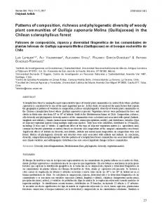
Supplementary Figure 1: Overview of the location and spread of sampling sites. From left to right: mediterranean climate zone of Australia, California, Chile and South-Africa. Below: illustration of the nested sampling performed in each quadrat and each Mediterranean-type region except California.
California
Australia
South‐Africa
Chile
California
Australia
South‐Africa
Chile
90
km
Nested
sampling
performed
in
each
of
the
20
x
20
m
scale
quadrats
in
Chile,
South‐Africa
and
Australia
2.5
m
7.5
m
20
m
20
m
4
Supplementary Figure 2: Combined phylogeny (i.e phylogeny of all 538 species combined). In yellow: species collected in the kwongan (Australia). In red: species collected in the chaparral (California). In blue: species collected in the matorral (Chile). In green: species collected in the fynbos (South-Africa). Phylogeny plotted using iTOL (http://itol.embl.de/index.shtml). protea amplexicaulis protea laurifolia protea nitida protea repens protea scorzonerifolia
protea acaulos adenanthos cygnorum isopogon spwatheroo isopogon tridens
is ro go au m is s hy isc lepi ich rvira ns a ud cu pe at ro hy ga s ca er isc pis lepi is om cens a le at ep gl es ro hyro ol ia rg ar isc chyr ow ia s vi is en ow oi om illd w illden nn w ca
hy
isc
petrophile shuttleworthiana petrophile scabruiscula petrophile pilostyla a petrophile macrostachy petrophile linearis dii drummon petrophile brevifolia petrophile i rmum wycherly conospe dis rmum stoecha conospe hyllum brachyp ermum boreale conosp ermum conosp latum canicu ermum osa conosp hea spinul ia synap latifol stirlingia yana dra lindle tata dryan dra triden a dryan leworthian dra shutt dra nivea dryan a dryan erian sia hook ziesii bank sia men na bank ollea sia cand nuata bank atte banksia elegans ksia na ban inca ksia sa ban gros ksia ata ban inul a unc eae greville a synaph iana greville ttleworth cata a shu a sac um ville ville gre gre ustifoli ra ang ltiflo lum tia mu icea me xylo lamber ea ser ta hak trifurca lia ea cifo hak rus ta ea stra hak pro ema ea hak lyanth bba po ea a en tat hakea kea cos a ha an kea ha ndolle ha ca rhync lia kea ilo llifo is ha a ps be ke a fla trinerv s ha ke mi ia ha on filifor is rso ia icular pe ta on ma rso ia ac co arpa pe on ia rso is on hic pe ns nc rso pe cyna cape tha a ian ida ge ltonia las rig s an str know matis con en luc ius cle rome rtus enar a nd rp de ocho s ar a ca mn ortu acro teat ia ac ow m tha ch br no gia en eus gia tham ele ele willd gent rcus s cu s ar bifu ua dis cu io cern ri be st po dis re oha sie ina hy po s er yp a hy ab lepi ss dian st
ch us qu pu ea pu pu ya cum co in bo ya be ya gi ch er ba rte ile ulea i wa boba rtia ns ro wa tson rtia orie nian is nt ts on ia m glad alis a ia ar bo gina iata rb on ta irid ica irid sp ar 3 ist ea irid sp2 ar ist ea capit sp1 af bu bu at xa lbi lbi rican a nth ne ne orrh lla lla a gr sp oe xa ac as nthor a drum alo ilis pa e rhoe ra mo sp a pr nd as gus pa ru eis ii as pa ragus bicun sii rag du lig um cry us afr nosu s be s llu ptoca ica lar rya nus ia ca alb pe um liforni a us bo ca ldu s
leucospermum calligerum paranomus lagopus serruria acrocarpa serruria effusa leucadendr on glaberrimu m leucadendron pubescen s leucadendron rubrum leucadendron salignum leucadendron spissifolium hibberti a hyperic oides hibbert ia crassif olia hibbert ia gnanga ra hibber tia huege lii hibbe rtia polys tachya nuytsia floribu nda osyris comp ressa thesi um aggr thesi egatu um m thesium hispidulum sp1 thes ium sp2 thes ium sp3 thes ium stric mue tum hlen bec ptilo tus stirli kia has tulata mac ngii arth uria ech aus inop drosan sis chil tralis ens them ere is um psia caly sp gale cina nia afri osc ularia cana lam sp pra nth lam us pra cae nth lam spitos us pra coc nth lam cineus us us pra em nth rus arg us chi ina a sp1 rus tus chi geminif a rus lora chi sp1 a rus chi sp3 carpe a sp6 nte my ria rsi ne califo dio afr sp rni ica yro eu ca na cle s a tom glabra an de en cro rso tos nia nin a lys he ine ia arcto ma kingia terop hy co sta ciliat na lla no ph um ste co ylo no as ste phium s vis tro as lom phium ma cida tro gn as lom a mi pr um tro cro eissii a as do tro loma gla leu lom sto uces nta leu copo a xe m ce ro arrh ns leu copo go ph en n pla leuc copo go yll a um nif go n le oli uc opog n affo us ldf le uc opog on allitti iel le dii uc opog on cono i er op cr og on ph as step er ica sif on ar hi ica er lo tic sp yll ru oide er ica bico ular re osta s s ng ch er ica cerin lor is el io ys er ica cocc th id ic es a faus inea oide hi s sp ta id ul a
1
is al qu ae in da a luci flora ii ic et er ica nudi en er ica pluk ula id er ica rig rrata ia er ica ol se m er icu ica taxif rn e er ica totta ria lifo thea ca er m us ica vis n ca ro os hyllu er do yo tic ica er dict mon fru ucop us io er oste mon gla otom lob oste mon trich lob oste mon ifera ccea lob oste bacc maco m nia sper ini lob icu iro ata ch ania ne alp gin thiop s log mo ia va m ae ide tum lio ca lar mu ga se ula ercu sper ath ea um op erm um sp yllac tho sp an ph erm tho sp caryo ensis an tho nia an s arv nti i mo olvulu rqu tosum pa nv co um tomen s str en ce is um lan pens cend sa so a ca ria as ymbo a ole ola ia cor rsiflor calce lar thy ceo cal laria viflora ceo bre cal lla lis kie na ona kec africa ridi a cta ofti a me s stri nso cilis psi alo gra ario bul glo selago enia udo rad pse mic ius s go dub oide sela on gon rod mic on poly niata rod mic ria laci guinea dula san glan che ban hyo ia sp ata igen hem sis spic i physop bartlingi are odia vulg pityr rubium sii mar gillie a reja iopic satu aeth hys or stac bicol teucrium mensis a sono aerulea salvi na−c africa salvia ulis albica salvia illinita a lonia escal pulverulent lonia escal nosa ia lanugi berzel pta interru lonicera ii sia huegel xantho rhiza sp anneso teinii trifida lichtens m num galbanu peuceda centella cordata centella debilis centella montana centella sp1 centella villosa wahlenbergia sp1
dav daviesia iesia triflo daviesia podoph ra ylla ped unculat davi esia nudifloraa davi esia incra davi ssat esia a diva davie sia decu ricata gomp holob gomp ium aristarrens holob tum ium tome gomp holob ium shutt ntosum bossiaea leworthii erioca rpa isotro pis cunei folia indigo fera sp2 indigof era sp1 indigof era digitata vicia sativa sophora macroca rpa aspalath us tridentat a aspalathu s ternata aspalathus retroflexa aspalathus pigmentosa aspalathus perfoliata
aspalathus pendulina aspalathus neglecta aspalathus lanata aspalathus heterophylla aspalathus cordata
lobelia excelsa lobelia polyphylla lobelia pinifolia goodenia coerulea lechenaultia linarioides
aspalathus ciliaris rafnia amplexicaulis acacia longifolia acacia caven
verreauxia reinwardtii dampiera incana dampiera linearis
acacia pulchella acacia lasiocarpa acacia barbinervis acacia auronitens acacia stenoptera acacia sessilis
scaevola canescens scaevola phlebopetala scaevola repens
eriophyllum confertiflorum baccharis linearis centaurea calcitrapa flourensia thurifera unknown unknown podanthu s mitiqui arctopus echinatu s erioceph alus africanu s haploca rpha lanata phaner ogloss a bolusii genusd d
acacia blakelyi jacksonia restioides nutans jacksonia hakeoides jacksonia a a floribund jacksoni e spe genussp arborea adesma alyx a trichoc mirbeli ia biloba criston are ema acicul choriz pifolia tia hysso ria mural tia heiste mural losa ltia angu mura rtum a confe ega sperm come a calym sperm osum acer come rma eana comespe gala papp ini garc poly gala poly naria ns aja sapo quill esce pub osa phylica plum s lica erbi phy imb lica elsa phy exc lica es phy roid tand osa cryp call lica a lica phy ifoli phy bux es lica phy ridioid s gen a spy ndr a pun tha crypta ptandr rian cry a my ermis ndr cod us pta leu eat cry hus is cun not hus trinerv cea ra not cea trevoa us rub ia ifol mn rha us ilic e tial no mn rha mile um hu em is lar nth um na em stipu ia ste nth s erv na alu uin ea ste ph inq seric a ce qu ho oli tia ea tric a for ruscif en qu gu clif tal pin lia rtia ifo pro cliffo rtia lygon ipera cliffo po jun ata rtia rtia atr ga ffo ffo rtia lon cli cli ffo tum cli ia ob ula ata ck cic ne a ge a fas argin los ka s lio de tom us em fo loi ya os un tia en ba betu ch pr ad ta ilis ae s m os pu am ar micr a hu rrata ch rin se olia rcoc a ce uarin ua ella cif ni as ocas mor quer slize gii oc all wi llo s all ella s pi or cu s ke le sp m er cu so s ry qu er tia qu s ch clu oide es cu on id er lyg no rosa qu po ater be anii tu rm al tia clu utia bia bu or bia cl ph eu phor
m on m otax on st co otax is gr ac llig an hy ua is br di st ja ac flo hy vio em od te ra on el ba la or at as de nt ax ife a tru hu cu illa ra m s ay s tri ca mbe ris cu lyc te ns ca nu sp ss s id inus ou ine oleo atus sia pe id es ra sc ro ro op gua ep ep ar rh us era era ia rh us tom fulvu sp rh us en sc ro yto to m sm ph sa rh arini ylla us rh fo us rim lia
lae os a rhus vig ata rh inc rhus us gla isa rhu s an dis uca se rhu gusti cta he eri s trilob folia a nd lithrea argen ata ron tea div ca schin ers ustic ilo a scu us lat bum lus ifo califo lius ea an rni a osm gustif a virg olia ag agath athosm ata aga a sp tho osma sm aga a cre salina tho sm a cap nulata aga tho ens sm is diosm diosm a bifi a acm a hirs da uta aeo ade phy ade nandra lla nan villo dra sa phil othe coriace ca a boronia spicata stru ram thio osa la stru thiola tetralepi stru thiola linearilob s dod a struthiol ecandra a gnid ia tome ciliata gnid ia inco ntosa nspi lachn cua aea uniflo lachn ra aea capit pass ata erina trunc passe rina filiformata pimelea is angu stifoli herma nnia scabr a herma a nnia hysso pifolia herma nnia angula ris hermannia alnifolia lasiopetalum drumm lasiopetalum ondii fremonto lineare dendron californic um heliophila subulata gyrostem on subnudus darwinia speciosa darwinia pauciflora
melaleuca zonalis melaleuca subtrigona
melaleuca leuropoma melaleuca trichophylla
eremaea hadra eremaea eremaea pauciflora eremaea violacea calytrix flavescens calytrix strigosa calytrix depressa calytrix leschenaultii calytrix sapphirina calytrix sp1 calytrix sp2 calytrix superba eucalyptus todtiana
darwinia neildiana baeckea grandiflora baeckea camphorosmae
ae
na
ath
ico de
do
ag
tox
do
er oc
pt
stac
kh
eu
ca pi io th ae sca ta be fu ca a tri os oe st oebe in um a st oebe pl 1 gu be sp st bi m oe be sp2 st am ru oe be e pe ides st oe ogyn as va halo st fla on ch tri axet pha gnap ta m an ncar pha virga um ifloru isp dr cr sy ncar pha ar um cylin osum um sy ys nc th m sy lichr ysum cy an um dasy ata he lichr ys he lichr um delic ys hr he um sp1 lic ys hr he um sp3 lic ys he hr um sp4 tum lic lla he hrys um ium ste lic fol he eti hrys um lic ter he hrys m lic su he hry arum lic a am he lat zlii es roe orbicu ulatus rib a es on nic rib ed pa urpure tyl on co od atrop ec ta tyl ssula dejec ularis la cra cic ssu la fas ltiflora cra lis ssu la mu dicau cra ssu cra la nu ovata ssu cra la ob ssu a cra la sp ssu crenat ullatum cra ea cuc ian um eni viv oni how m arg um bru pel oni sca arg um s pel oni arg elegan ervis pel alum rtia trin lus ufo nus thopet pha bea otham ma xan phyroce con lym por oca rpus hyp oca lius mat phy sa us filifo anth ia obtu ndrum pile gen oliga ceu ns um myr esce erm spin m leptosp mum igatu sper laev lepto mum ta sper lucra lepto invo a ltzia eabb scho spen ra ltzia ellife scho umb sus ltzia s scho us torulo ermu hamn arosp calot s bleph amnu rifidus caloth s quad amnu ineus caloth s sangu amnu caloth densiflora verticordia grandis rdia vertico lia rdia ovalifo vertico era rdia pennig vertico arpa a asteroc eremae ioides beaufort eremaea lada ectadioc
genus ff genus ll genus pp genu ssp2 sp2 genu ssp10 sp10 genu ssp1 2 sp12 genu ssp6 sp6 eupa toriu m glech eupa onop toriu m salv hyllu dimo m ia rpho thec dimo a trag rpho us thec arct a wall otis belli arct difolia iana otis sem prou ipap stia prousti cinerea posa a pug pro usti ens corymb a pyr ifoli a ium cor ymbiu sp2 cor m sp3 ym biu cor m sp4 ym biu ost m eos per sp5 chr mu ysa m jun nth trip em ter ceu heter is tom oides m mo ent ole cul nilifera lum pis alie osa ia cili be na rkh aris eya be rkh eya barba eu ryo ta ps herba eu ryo ab rot cea ps eu an ryo sp ifolius ec oth ps ten iosiss on oth na uis im on pa se rvi simus us na ne flo cio quinq ra se ne cio aloide uede se ne nta s cio sp ch ta rys ve fel sti ici oc pte a fili oma tum pter ronia folia ciliat a ca pter on ia mp cin os on ho ia m at ito inc erea rata ha ps an hy na is a ur men sia pinna sin ole trifu tifi ur sin ia pa pis rcat da ur sin ia sp leac crith a oe ia 1 ea mifo m dera se lia et ric m al as squa ea el etal ia rro yt el ro asia de sa el ytro papp fast nsa yt ro papp us igia pa pp us gnap ta us hisp ha in tri idus loid ca es ta
5
communities from the matorral and chaparral. These tendencies did not cause major deviations of the observed PD-area relationship from that expected under the random assembly hypothesis (Figure 3 from the main text, see also Appendix S4). Results obtained using other phylogenetic diversity metrics, namely the mean pairwise distance (MPD), which measures the mean phylogenetic distance among all pairs of species in the community and the mean nearest neighbor distance (MNND), which measures the mean phylogenetic distance to the nearest relative for all species in the community (Webb et al., 2002), were qualitatively similar (results not shown). Using a similar approach, we tested for potential deviations from the random assembly hypothesis across pairs of samples (within region), at the sample size used in the paper (i.e. the 20 x 20 m scale). We ranked the χP D observed between two samples, one containing S1 species, the other containing S2 species, and the two sharing S1∩2 species within the χP D of 1000 community pairs assembled by randomly sampling S1 and S2 species in each regional phylogeny while keeping S1∩2 constant. The significance of the deviation from the random assembly model was then obtained by dividing the rank of the observed χP D by the number of observations (1001). A relative rank lower than 0.05 indicates communities that are significantly less phylogenetically similar than expected by chance given the number of species present within each, and shared between, the two communities. A relative rank greater than 0.95 indicate communities that are significantly more phylogenetically similar than expected by chance given the number of species present within each, and shared between, the two communities. With this level of significance, only a few communities deviated significantly from the random assembly hypothesis, except in the fynbos, where there was a marked tendency for pairs of communities to be more similar than expected by chance (Fig. S4). This tendency caused the observed decay in phylogenetic similarity to lie above (i.e. have greater similarity values) the one expected under the random assembly hypothesis (Figure 4 from the main text, see also Appendix S4). Our result that the PD supported by communities, and shared across communities, is most 6
0.0
0.2
0.4
0.6
0.8
1.0
4 0
4 0
0
4
8
kwongan 20m
8
kwongan 7.5m
8
kwongan 2.5m
0.0
0.2
0.4
0.6
0.8
1.0
0.4
0.6
0.8
1.0
0.4
0.6
0.8
1.0
0.6
0.8
1.0
8 0 0.0
0.2
0.4
0.6
0.8
1.0
0.0
0.2
0.4
0.6
0.8
1.0
rank of observed versus random
chaparral 20m 8
rank of observed versus random
0.4
4
1.0
0.2
0
0.8
0.0
4
8 0 0.6
1.0
matorral 20m
4
8
0.4
0.8
8 0.2
matorral 7.5m
4
0.2
0.6
0 0.0
matorral 2.5m
0.0
0.4
4
8 4 0.2
0.2
fynbos 20m
0
4 0 0.0
0.0
fynbos 7.5m
8
fynbos 2.5m
0
number of communities
number of communities
number of communities
Supplementary Figure 3: Random assembly within communities in the Mediterranean data. Histograms report the number of communities falling in a given rank class (relative rank as defined above). Communities falling on the left of the blue line are less phylogenetically diverse (i.e. have a smaller PD) than expected by chance given their species richness, and significantly so when they fall on the left of the first orange line. Communities falling on the right of the blue line are more phylogenetically diverse (i.e. have a higher PD) than expected by chance given their species richness, and significantly so when they fall on the right of the second orange line. From left to right: data collected at the 2.5 x 2.5 m, 7.5 x 7.5 m, and 20 x 20 m scales.
0.0
0.2
0.4
0.6
0.8
1.0
rank of observed versus random
7
Supplementary Figure 4: Random assembly across communities in the Mediterranean data. Histograms report the number of community pairs falling in a given rank class (relative rank as defined above). Communities falling on the left of the blue line are less phylogenetically similar than expected by chance given their species richness and turnover, and significantly so when they fall on the left of the first orange line. Communities falling on the right of the blue line are more phylogenetically similar than expected by chance given their species richness and turnover, and significantly so when they fall on the right of the second orange line.
60 40 20 0
20
40
60
fynbos
0
number of community pairs
kwongan
0.0
0.2
0.4
0.6
0.8
1.0
0.0
0.2
0.6
0.8
1.0
0.8
1.0
60 40 20 0
20
40
60
chaparral
0
number of community pairs
matorral
0.4
0.0
0.2
0.4
0.6
0.8
1.0
0.0
rank of observed versus random
0.2
0.4
0.6
rank of observed versus random
8
often not significantly different from expected under the random assembly hypothesis is conservative. Applying a Bonferroni correction in order to account for multiple testing (per continent, we performed 30 tests within communities, and 435 tests across communities tests) would reduce the number of communities or pairs of communities deviating significantly from this hypothesis.
Appendix S3: Species-PD relationship of the combined phylogeny and sensitivity analysis Species-PD relationship of the combined phylogeny
Fig. S5 illustrates the species-PD
curve of the phylogeny of the 538 species combined, and how it compares to regional speciesPD curves. The figure shows that the scale invariant species-PD curve holds on the combined phylogeny, with a z* exponent similar to exponents observed in regional phylogenies.
Sensitivity analysis
To test the robustness of the species-PD curves and related exponents to
uncertainty in the phylogeny, we separately explored the effect of polytomies and of the node age assignment algorithm. Code for these analyses is available at www.schwilk.org/research/data.html.
Polytomies An analysis of the effect of a lack of resolution on measurements of phylogenetic diversity, performed on simulated phylogenies, has shown that phylogenetic diversity is particularly sensitive to a lack of resolution basally (Swenson, 2009). Here, we were interested in the effect of missing resolution in our specific data, and on the specific patterns investigated in the paper (in particular the species-PD curve). To explore the effect of polytomies, we conducted the following procedure for each phylogeny (the combined phylogeny and the four regional phylogenies): 1) we created a set of 1000 alternative versions of the full unpruned phylogeny (i.e. angiosperm backbone tree + 538 species) and then ran the modified BLADJ algorithm on each of these to assign branch-lengths by dating undated nodes. For each of these 9
103 102.5 ●
● ● ● ● ● ● ● ● ● ● ● ● ● ●
● ● ● ● ● ● ● ● ● ● ● ● ● ●
● ● ● ● ● ● ● ● ● ● ● ● ● ● ●
● ● ● ● ● ● ● ● ● ● ● ● ● ● ● ● ●
● ● ● ● ● ● ● ● ● ● ● ● ● ● ●
● ● ●● ● ● ● ●● ● ● ● ● ● ●● ● ● ● ● ● ●● ● ●● ● ● ● ●
● ● ● ● ● ● ● ● ● ● ● ● ●
● ● ● ● ● ● ● ● ● ● ● ● ● ● ●
● ● ● ● ● ● ● ● ● ● ● ● ● ● ● ●
● ● ● ● ● ● ● ● ● ● ● ● ●
● ● ● ● ● ● ● ● ● ● ● ● ●
● ● ● ● ● ● ● ● ● ● ● ●
● ● ● ● ● ● ● ● ● ● ● ●
● ● ● ● ● ● ● ● ● ● ●
100
● ● ● ● ● ● ● ● ●
● ● ● ● ● ● ●
● ● ● ●
● ● ● ●
●●
●
●
global z*= 0.71 Australia z*= 0.64 South−Africa z*= 0.68 Chile z*= 0.73 California z*= 0.74
●
●
100.5
● ● ● ● ● ● ● ● ● ● ●
● ● ● ● ● ● ● ● ● ● ●
● ● ● ● ●● ● ● ● ● ●● ● ● ● ● ● ● ● ●
● ● ● ●
●
102
PD (Myrs)
103.5
104
Supplementary Figure 5: Species-PD relationship of the combined phylogeny (in black) and comparison with the species-PD curve of each regional phylogeny. Data points (black circles) are the results of 100 simulated random samplings across the tips of the combined phylogeny. Lines are power-law fits across the data (data points corresponding to regional phylogenies not shown for clarity). The species-PD curve of the combined phylogeny is well approximated by a power-law curve with an exponent similar to those observed in regional phylogenies.
101
101.5
species richness
10
102
102.5
randomizations, we conducted a rarefaction analyses as described in the main text with 100 random draws for each species richness value. The random resolution of polytomies followed by BLADJ branch-length assignment tended to curve the power-law species-PD curve downward towards the end of the sampling procedure (i.e. when almost all species were included), and consistently lowered z* values (Fig. S6). Randomly resolving polytomies pushed undated nodes towards the tips of the phylogenies. Deviations from the pattern observed without randomly resolving polytomies were the lowest in the Californian dataset where all nodes were resolved, and the largest in the Australian and South-African datasets where many polytomies remained. In the global phylogeny, the z* value was 0.71 without resolution, and the mean over 100 random resolutions was 0.65. In all phylogenies, the power-law approximation remained relevant after random resolution. In particular, the power-law always provided a better fit than the previously proposed logarithm (Nee & May, 1997) (black versus blue fit in Fig. S.6). Deviations from z* values obtained without random resolutions were always less than 0.1 unit. Hence, the presence of polytomies in the phylogenies does not compromise the main approach and conclusions of our study.
BLADJ branch-length assignment To test the sensitivity of the relationships to the BLADJ evenly-spaced node age method, we generalized the node dating algorithm to allow undated nodes to be assigned dates according to any normalized age distribution. We explored two variations. In the first branch-length sensitivity analysis, instead of assigning node ages deterministically and evenly, node ages were assigned from a uniform random distribution with bounds set by fixed ages of ancestors and descendants. Using this method, we explored a set of 1000 phylogenies that varied in branch-length assignment for each topology. As expected, using a
11
Supplementary Figure 6: Robustness of the power-law shape of species-PD curves, and sensitivity of z* values, to random resolutions of polytomies followed by BLADJ branch-length assignment. For each dataset, we constructed 1000 randomly resolved phylogenies. On the left: data points (black circles) are the results of 100 simulated random samplings across the tips of one (randomly chosen) of the 1000 randomly resolved phylogenies. The black line is the power-law fit across the data points. The orange line is the power-law fit corresponding to the original unresolved phylogeny (data points not shown for clarity). This line is barely visible in the matorral and chaparral, because randomly resolving polytomies in the corresponding phylogenies had very little effect on the species-PD curve. Note that deviations from the orange line in the kwongan and fynbos do not reflect deviations from the power-law (deviations from the black line would), but rather deviations from the species-PD curve obtained without randomly resolving the polytomies. The blue line is the best-fit logarithm, shown for comparison with previous literature (Nee & May, 1997). The power-law (black line) provides a much better fit than the logarithm (blue line). On the right: Distribution of z* values for the 1000 randomly resolved phylogenies. The red line indicates the z* value corresponding to the original unresolved phylogenies. Randomly resolving polytomies pushed undated nodes towards the tips of the phylogenies, tended to curve the power-law species-PD curve downward towards the end of the sampling procedure, and consistently lowered z* values.
102.5
● ● ●
z*= 0.6 z* = 0.65
102
●
● ● ● ● ● ● ●
0.56 102.5
100
104
Matorral
101
101.5
102
Chaparral
●
● ● ● ● ● ● ● ● ●
102.5
z*= 0.7 z*= 0.73
● ●
102
●
● ● ● ● ● ● ● ● ● ● ●
z*= 0.73 z*= 0.74
0.69 100
100.5
101
101.5
102
species richness
102.5
100
100.5
101
101.5
0.64
0.66
0.62
102
102.5
12
0.70
Matorral
Chaparral
0.70
0.71
0.72 z*
species richness
0.66 z*
150 Frequency
● ● ● ● ● ● ● ● ● ● ● ● ● ● ● ● ● ● ● ● ● ● ● ● ● ● ● ● ● ● ● ● ●● ● ● ● ● ●● ● ● ● ● ● ● ● ● ● ● ● ● ●● ● ● ● ● ● ● ●● ● ● ● ● ● ● ● ● ● ● ● ● ● ●● ● ● ● ● ●● ● ● ● ● ● ● ● ● ● ●
102
0.62 z*
50
102.5
103
0.60
0
103
0.58
102.5
103.5 ● ●● ● ● ● ● ● ● ● ● ● ● ● ● ● ● ● ● ● ● ● ● ● ● ● ● ● ● ● ● ● ● ● ● ● ● ● ● ● ● ● ● ● ●● ● ● ● ● ● ● ● ● ● ● ● ●● ● ● ● ● ● ● ● ● ● ●● ● ● ● ● ● ● ● ● ● ●● ● ●● ● ● ● ● ● ● ● ● ● ●● ●● ● ● ●● ● ● ● ● ● ● ● ● ● ●● ● ● ● ● ● ● ● ● ● ● ● ● ●
PD (Myrs)
PD (Myrs)
103.5
100.5
0.74
200
102
Frequency
101.5
50
101
0
104
100.5
100
100
200
Frequency
250 150
Frequency
z*= 0.64 z*= 0.68
●
102
50 100
● ● ● ● ● ● ● ● ●
103
Fynbos
0
●
● ● ● ● ● ● ● ● ● ● ● ● ● ● ● ● ● ● ●
103.5
●● ● ● ● ● ● ● ● ● ● ● ● ● ● ● ● ● ● ● ● ● ● ● ● ● ● ● ● ● ● ● ● ● ● ● ● ● ● ● ● ● ● ● ● ● ● ● ● ● ● ● ● ● ● ● ● ● ● ● ● ● ● ● ● ● ● ● ● ● ● ● ● ● ● ● ● ● ● ● ● ● ● ● ● ● ● ● ● ● ● ● ●● ● ● ● ● ● ● ● ● ● ●● ● ● ● ● ● ● ● ● ● ● ●● ● ● ● ● ●● ● ● ● ● ● ● ● ● ● ●● ●● ● ● ● ●● ● ● ● ● ● ● ● ● ● ● ● ● ●● ● ● ●● ● ● ● ● ● ● ● ● ● ● ● ● ● ● ● ● ●
100
102.5
● ● ● ● ●● ● ● ●● ● ● ● ● ● ● ● ● ● ● ● ● ● ● ● ● ● ● ● ●● ● ● ● ● ● ● ● ● ● ● ●● ● ●
Kwongan
Fynbos
50
103
● ●● ● ● ● ● ● ● ● ● ● ● ● ● ● ● ● ● ● ● ● ● ● ● ● ● ● ● ● ● ● ● ● ● ● ● ● ● ● ● ● ● ● ● ● ● ● ● ● ● ● ● ● ● ● ● ● ● ● ● ● ● ● ● ● ● ● ● ● ● ● ● ● ● ● ● ● ● ● ● ● ● ● ● ● ● ● ● ● ● ● ● ● ● ● ● ● ● ● ● ● ● ● ● ● ● ● ● ● ● ● ● ● ● ● ● ●
PD (Myrs)
103.5
PD (Myrs)
104
Kwongan
0
104
0.73
0.74
0.725
0.730
0.735 z*
0.740
uniform distribution of ages instead of an evenly-spaced distribution did not change the shape of curve; it increased the variance in z* values, but did not drastically change mean values (Fig. S7). Supplementary Figure 7: Robustness of the power-law shape of species-PD curves, and sensitivity of z* values, to branch-length assignment using a random uniform distribution of node ages instead of evenly spacing nodes. For each dataset, we constructed 1000 phylogenies with undated nodes assigned ages from a uniform distribution. On the left: data points (black circles) are the results of 100 simulated random samplings across the tips of one (randomly chosen) of the 1000 random phylogenies. The black line is the power-law fit across the data points. The orange line, which represent the the power-law fit corresponding to the original phylogeny, can barely been seen due to the robustness of the species-PD curve to the method of branch-length assignment. The blue line is the best-fit logarithm, shown for comparison with previous literature(Nee & May, 1997). On the right: Distribution of z* values for the 1000 random node age phylogenies. The red line indicates the z* value corresponding to the original phylogenies. Uniformly distributing nodes does not significantly change the shape of the species-PD curve, and does not greatly influence mean z* values. Rather, this method increases the variance in z* values.
102
●
● ● ● ● ● ● ● ● ●
Frequency 0.60
102
102.5
100
104
●
10
100.5
101
101.5
0.70
0.75
0.68
102
species richness
102.5
0.70
0.72
0.74
z*
Matorral
Chaparral
0.76
200
z*
●
● ● ● ● ● ● ● ● ● ●
●
z*= 0.74 z*= 0.74
2
10
Frequency
150
● ● ● ● ● ● ● ● ● ● ● ● ● ● ● ● ● ● ● ● ● ● ● ● ● ● ● ● ● ● ● ● ● ● ●● ● ● ●● ● ● ● ●● ● ● ● ● ● ● ● ● ● ● ●● ● ● ●● ● ● ● ● ● ● ●● ● ● ● ● ● ● ●● ● ● ● ● ● ● ● ● ●
100
103
0.70 100
0.65
102.5
Chaparral
102.5
z*= 0.74 z*= 0.73
2
102
50
● ● ● ● ● ● ● ● ●
101.5
0
102.5
101
103.5
●● ● ● ● ● ● ● ● ● ● ● ● ● ● ● ● ● ● ● ● ● ● ● ● ● ● ● ● ● ● ● ● ● ● ● ● ● ● ● ● ● ● ● ● ●● ● ● ● ● ● ● ●● ● ● ● ● ● ● ● ● ● ● ● ● ● ● ●● ● ● ● ● ● ● ● ●● ● ● ● ● ● ● ●● ● ● ● ● ● ● ● ● ● ●
PD (Myrs)
103
100.5
Frequency
101.5
Matorral
103.5
PD (Myrs)
101
50
104
100.5
0
100
100 150 200 250
250 200 150 100
Frequency
z*= 0.69 z*= 0.68
102
Fynbos
50
102.5
z*= 0.68 z* = 0.65
Kwongan
● ● ●
0
● ● ● ● ● ● ● ● ● ●
103
● ● ●
100
100.5
101
101.5
102
102.5
150
●
103.5
● ● ● ● ● ● ● ● ● ● ● ● ● ● ● ● ● ● ● ● ● ● ● ● ● ● ● ● ● ● ● ● ● ● ● ● ● ● ● ● ● ● ● ● ● ● ● ● ● ● ● ● ● ● ● ● ● ● ● ● ● ● ● ● ● ● ● ● ● ● ● ● ● ● ● ● ● ● ● ●● ● ● ● ● ● ● ● ● ● ●● ● ● ● ● ● ● ● ● ● ●● ● ● ● ●● ● ● ● ● ● ● ●● ● ● ● ● ● ● ● ● ●● ● ● ● ● ●● ● ● ● ● ● ● ● ● ● ● ● ● ● ●
100
102.5
● ● ● ● ● ● ● ● ● ● ● ● ● ● ● ● ● ●● ● ● ● ● ● ● ●● ● ● ● ● ● ● ● ● ●● ● ●● ● ● ● ● ● ● ●
Fynbos
50
103
● ● ● ● ● ● ● ● ● ● ● ● ● ● ● ● ● ● ● ● ● ● ● ● ● ● ● ● ● ● ● ● ● ● ● ● ● ● ● ● ● ● ● ● ● ● ● ● ● ● ● ● ● ● ● ● ● ● ● ● ● ● ● ● ● ● ● ● ● ● ● ● ● ● ● ● ● ● ● ● ● ● ● ● ●
●● ● ● ● ● ● ● ●
PD (Myrs)
103.5
PD (Myrs)
104
Kwongan
0
104
0.74
0.78 z*
0.82
0.60
0.65
0.70
0.75
0.80
z*
species richness
In the second branch-length sensitivity analysis, we explored node age distributions skewed towards either the root or the tips. For this analysis, node ages were drawn from a truncated
13
exponential distribution (again with bounds set by fixed ancestor and descendant ages). We defined a parameter, α, to control the amount of skewness. The truncated exponential parameter, λ, was then calculated from α: λ =
1 (Aa α
− Ad ), where Aa and Ad are the ages of the fixed
ancestor and descendant. Lower absolute values of alpha result in greater skew. We defined the algorithm such that λ can be relative to the ancestor age (positive alpha values, skewed toward root, resulting in longer branches at the tips) or the descendant age (negative alpha values, skewed toward tips, resulting in longer branches toward the root). We explored 1000 randomizations for each of six different truncated exponential distributions: three skewed towards the root with α values of 0.8, 0.6, and 0.2 and three skewed towards the tips with α values of 0.8, -0.6, and -0.2. We then ran the full rarefaction analysis on each of these phylogenies. The power-law shape of the curve was only affected for strong skews (|α|=0.2) and more sensitive to a skew towards the tips than towards the root (Fig. S8). As expected, z* values decreased when nodes were distributed towards the tips, and decreased when nodes were distributed towards the root. Deviations from initial z* values were always less than 0.1 unit and did not compromise the main approach and conclusions of our study (Fig. S9).
Appendix S4: Statistical tests relevant to spatial phylogenetic diversity patterns and predictions This section describes the statistical tests that we used to: 1) test the ability of the random assembly process to reproduce observed spatial phylogenetic diversity patterns (thereafter referred to as Test 1), and 2) test the accuracy of our spatial phylogenetic diversity theory predictions (Test 2). Test 1 is different from the tests performed in Appendix S2. In Appendix S2, we tested for potential deviations from the random assembly model at the level of individual communities (Fig. S3) or pairs of communities (Fig. S4). Here, we test for potential deviations from the random assembly model across communities, to assess if the observed spatial patterns deviate from
14
Supplementary Figure 8: Robustness of the power-law shape of species-PD curves to branchlength assignment using a distribution of node ages skewed towards the root or the tips instead of evenly spacing nodes. α values determine the direction and strength of the skew. Top row: distribution skewed toward the root (i.e. undated nodes are pushed towards the root). Bottom row: distribution skewed towards the tips (i.e. undated nodes are pushed towards the tips). From left to right: increasing skew. For each α value, we constructed 1000 phylogenies in which node ages were drawn from a truncated exponential distribution. The power-law shape is robust. Results - shown here for the combined phylogeny - were similar for regional phylogenies.
103
● ● ● ● ● ●● ● ● ● ● ● ● ● ● ● ●● ● ● ● ● ●● ●● ● ● ● ● ● ● ● ● ● ●● ● ● ● ●● ● ● ● ● ● ● ● ● ● ●
102.5 ●
102
● ● ● ●
● ● ●
● ● ● ●
104
103.5
103
102.5 ●
z*= 0.73 z*= 0.71
● ● ● ● ● ● ●● ● ● ● ● ●● ● ● ● ● ●● ●● ● ●● ● ●● ● ● ● ● ● ● ●● ● ● ● ● ● ● ● ● ● ● ● ● ●
103
102.5 ●
102
103.5
103
●
z*= 0.76 z*= 0.71
100 100.5 101 101.5 102 102.5
104
103.5
103
102.5 ●
● ● ● ● ● ● ● ● ● ● ● ●
● ● ● ● ● ● ● ● ● ● ● ● ● ●● ● ● ● ● ● ● ●● ● ● ●● ●● ● ● ● ● ● ●● ● ● ● ●
● ● ● ● ● ● ● ● ● ●● ● ● ● ● ●● ● ● ●● ● ● ● ●● ● ● ● ● ● ● ● ● ●● ● ● ●● ●● ● ● ● ● ● ● ● ●● ●● ● ● ● ● ● ● ●● ● ● ●● ● ● ● ● ● ●● ● ●● ●● ● ●● ● ● ●● ● ● ● ● ●● ●● ● ● ●● ● ● ●● ● ●● ● ● ● ● ●● ●● ● ● ● ● ● ●● ● ● ● ● ●● ● ● ● ● ● ●● ● ●● ● ● ● ●● ● ● ● ● ● ● ●
● ● ●
100 100.5 101 101.5 102 102.5
100 100.5 101 101.5 102 102.5
15
104
103.5
103 ●
102.5
species richness
● ● ● ●
z*= 0.82 z*= 0.71
102
● ● ●
z*= 0.69 z*= 0.71
102
● ● ● ● ● ● ●
species richness α = − 0.2
● ● ●
z*= 0.71 z*= 0.71
species richness
● ● ● ● ●● ● ● ● ● ●● ● ● ● ● ● ● ● ● ● ● ●● ● ● ● ● ● ● ● ● ● ● ● ● ● ●● ● ● ● ●● ● ● ● ● ● ● ● ● ● ● ●● ● ● ● ● ● ● ● ●● ●● ● ● ● ●● ●● ● ● ● ●● ● ● ● ● ● ● ● ● ●● ● ●● ● ● ● ● ●● ● ● ●● ● ● ● ● ● ● ● ● ● ●● ●● ● ● ●● ● ● ● ● ● ●● ● ● ●● ●● ● ● ● ●● ● ● ● ● ● ● ● ● ● ●● ● ● ● ● ● ● ● ● ● ● ● ●
104
species richness α = − 0.6
PD (Myrs)
PD (Myrs)
103.5
● ● ●
100 100.5 101 101.5 102 102.5
species richness α = − 0.8
● ● ● ●● ● ● ● ●● ● ● ● ● ● ●● ● ● ● ● ● ●● ● ● ●● ● ●● ● ●● ●● ● ● ● ● ● ● ● ● ● ● ● ●● ● ● ● ● ●● ● ● ● ● ● ● ●● ●● ● ● ● ● ●● ● ● ● ● ● ● ● ● ● ●● ● ● ● ● ●● ● ● ● ● ● ● ● ●● ● ● ● ● ●● ●● ●● ● ● ● ● ● ● ● ● ●● ●● ● ● ● ●● ●● ● ● ● ● ● ● ● ● ● ●● ● ● ● ● ● ●● ●● ● ● ● ● ● ●● ● ● ● ● ●● ●● ● ● ●● ● ● ● ● ●● ● ● ● ● ● ● ● ● ●● ● ● ● ● ● ●
● ● ● ●
102.5
102
100 100.5 101 101.5 102 102.5
104
● ● ● ● ● ● ● ● ●● ● ● ● ● ● ●● ● ● ● ● ● ● ●● ● ● ●● ● ● ● ● ● ● ●● ● ● ● ● ●● ● ● ●● ● ● ● ● ● ●● ● ● ●● ● ● ● ● ● ● ● ● ●● ● ● ● ●● ● ● ● ● ● ●● ● ● ● ●● ●● ● ● ● ● ●● ● ●● ● ● ● ● ●● ●● ● ● ● ● ● ● ● ●● ● ● ● ● ● ●
α = 0.2 ● ● ● ●
PD (Myrs)
PD (Myrs)
103.5
● ● ● ● ● ● ● ● ● ●● ● ● ● ● ● ●● ● ● ● ● ● ●● ● ● ● ● ●● ● ● ●● ● ● ● ● ● ●● ● ● ● ● ●● ● ●● ● ● ●● ● ● ● ● ●● ● ● ● ●● ● ● ●● ●● ●● ● ● ● ● ● ● ● ● ● ●● ● ● ● ● ●● ● ● ● ●● ●● ● ●● ●● ●● ● ● ● ● ● ● ●● ● ● ●● ● ● ● ● ●● ● ● ●● ● ● ● ● ● ● ● ●● ● ● ●
● ● ● ● ● ● ● ● ● ● ●
PD (Myrs)
104
α = 0.6
PD (Myrs)
α = 0.8
●
102
● ● ● ● ● ● ● ● ● ● ● ● ● ●● ● ● ● ●● ● ● ● ●● ● ●● ● ● ● ●● ●● ● ● ● ● ● ● ● ● ● ● ● ● ● ● ● ●
● ● ● ●● ● ● ● ● ● ● ● ● ● ● ● ● ● ●● ● ● ●● ● ● ●● ● ● ● ● ● ● ●● ● ● ● ● ●● ● ●● ● ● ● ● ● ● ●● ● ● ●● ● ● ●● ● ●● ● ● ● ● ● ●● ● ● ●● ●● ●● ● ● ● ●● ●● ● ● ● ● ● ● ●● ● ●● ● ● ● ● ● ●● ●● ●● ● ● ● ● ● ●● ●● ● ● ● ● ● ●● ● ●● ● ● ● ● ● ● ● ●● ●● ● ● ● ● ● ● ● ●● ● ● ● ● ●● ●
z*= 0.66 z*= 0.71
100 100.5 101 101.5 102 102.5
species richness
Supplementary Figure 9: Sensitivity of z* values to branch-length assignment using a distribution of node ages skewed towards the root or the tips instead of evenly spacing nodes. α values determine the direction and strength of the skew. Top row: distribution skewed toward the root (i.e. undated nodes are pushed towards the root). Bottom row: distribution skewed towards the tips (i.e. undated nodes are pushed towards the tips). From left to right: increasing skew. For each α value, we constructed 1000 phylogenies in which node ages were drawn from a truncated exponential distribution. As expected, phylogenies with longer terminal branchlengths (top) have higher z* values, and phylogenies with shorter terminal branch-lengths (bottom) have higher z* values. Results - shown here for the combined phylogeny - were similar for regional phylogenies.
α = 0.2
0.70 0.72 0.74 0.76 0.78
80 0
0
0
20
20
20
40
60
Frequency
60 40
Frequency
40
Frequency
60
100
80
120
α = 0.6
80
α = 0.8
0.70 0.72 0.74 0.76 0.78
0.70
0.78 z*
α = −0.8
α = −0.6
α = −0.2 150
0.82
0.67
0.69
0.71
0.73
0
0
20
20
50
100
Frequency
60
Frequency
40
40
60
80
80
100
z*
0
Frequency
0.74
z*
0.66
z*
0.68
0.70 z*
16
0.64
0.66
0.68 z*
0.70
those expected under random community assembly. To perform Test 1, we compared observed curves to the 95% confidence envelopes of the curves obtained by simulations of the random assembly process (see below). To perform Test 2, we compared the predicted curves to these same confidence envelopes. Statistical tests related to PD-area curves To construct the 95% confidence envelope of the PD-area curve in a given Mediterranean region, we performed the three following steps: 1) we ran 1000 simulations of the random assembly process (keeping species richness constant) across all 30 samples at all scales, 2) we constructed the PD-area curve corresponding to each simulation by averaging, at each spatial scale, PD values across the 30 samples, and 3) we excluded, at each spatial scale, the 5% most extreme values. To test the ability of the random assembly process to reproduce the observed PD-area curve (Test 1), we compared this observed curve (obtained by averaging across the 30 samples at each scale) to the 95% confidence envelope of the PD-area curve. The observed PD-area curve (orange line in Fig. S10) fell within the 95% confidence envelope of the curve obtained under random assembly (black lines, Fig. S10). In agreement with the results found in Appendix S2 (Fig. S3), the observed PD tended to be lower than expected under random assembly in the kwongan (specially at the largest spatial scales) and fynbos (at all spatial scaes), and higher than expected under random assembly in the chaparral. None of these tendencies were significant. To test the accuracy of the PD-area predictions (Test 2), we compared the predicted curves (Equations 2 and 4 from the main text) to the 95% confidence envelope. The predictions from Equation 2 do not make the assumption that the species-area curve is power-law, whereas the predictions from Equation 4 do. The predictions from Equation 4 (blue dashed lines, Fig. S 10) were in good agreement with the predictions from Equation 2 (blue circles, Fig. S10),
17
demonstrating the validity of using the power-law to describe the species-area curve in our data. The predicted curves (blue circles and blue dashed lines) fell within the 95% confidence envelope obtained under random assembly (black lines, Fig. S10) in the kwongan and chaparral. In the fynbos, the predicted curves were close to the lower bound of the 95% confidence interval. This deviation was due in part to the fact that PD values were slightly lower than expected by chance, and it was also due to deviations from the power-law assumption for the species-PD curve in the fynbos. Regardless of these deviations, the predicted curves yielded a reasonable quantitative description of the data. Statistical tests related to the decay in phylogenetic similarity with geographic distance To construct the 95% confidence envelope of the phylogenetic distance-decay curve, we performed the three following steps: 1) we ran 1000 simulations of the random assembly process (keeping species richness and turnover constant) across all 435 sample pairs at the 20 x 20 m scale 2) we constructed the phylogenetic distance-decay curve corresponding to each simulation by pulling data points falling in 0.2 distance bins (on a log scale) 3) we excluded, in each bin, the 5% most extreme values. To test the ability of the random assembly process to reproduce the observed phylogenetic distance-decay curve (Test 1), we compared this observed curve (obtained by pulling data points falling in 0.2 distance bins, orange line in Fig. S11) to the 95% confidence envelope of the curve obtained under random assembly (black lines in Fig. S11). This comparison shows that the random assembly process tends to overestimate similarity values in the kwongan, and underestimate them in the fynbos, although this discrepancy is only significant at the smallest spatial separation in the kwongan. The fact that observed similarity values tend to be higher in the fynbos than expected under random assembly is in agreement with the results found in Appendix S2 (Fig. S4).
18
Supplementary Figure 10: Test of theory predictions for the PD-area relationship. The observed relationship (orange line) is in good agreement with relationships obtained under random assembly (95% confidence interval represented by black lines). The predictions from Equation 2 (blue circles) fail in the fynbos, mainly due to deviations from the species-PD curve powerlaw assumption. The predictions from Equation 4 (blue dashed lines) fail in the fynbos due to the previous failure of Equation 2. PD-area curves were obtained by averaging the data over the 30 samples at each spatial scale.
Kwongan
3.4
PD (Myrs)
●
3.2 3.0
●
●
2.8 2.6
1.0
1.5
2.0
2.5
Fynbos
3.4
PD (Myrs)
●
3.2
●
3.0 ●
2.8 2.6
1.0
2.0
2.5
Chaparral
3.4
PD (Myrs)
1.5
3.2 ●
3.0 ●
2.8 ●
2.6
1.0
1.5
2.0
area (m2)
19
2.5
Deviations between the observed and predicted (Test 2, Equation 6 from the main text) phylogenetic distance-decay curves occurred in the kwongan and fynbos (Figure 4 from the main document). These deviations from the observed phylogenetic distance-decay curves have three potential origins: 1) deviations linked to the random assembly hypothesis 2) deviations linked to the power-law approximation for species-PD curves (resulting in Equation 5 from the main text) 3) deviations linked to fitting a logarithmic curve to the species distance-decay relationship (resulting in Equation 6 from the main text). The first source of error has been discussed in the previous paragraph, and explains part of the deviations in the fynbos. To evaluate the second source of error, we compared predictions given by Equation 5 (blue circles in Fig. S11) to the 95% confidence envelope of the curve obtained under random assembly (black lines). This comparison reveals that a good part of the deviations observed in the fynbos is linked to the power-law assumption for the species-PD curve, which results in a consistent underestimation of phylogenetic similarity values. To evaluate the third source of error, we compared predictions given by Equation 6 (blue dashed lines; this equation assumes a logarithmic fit to the species distance-decay relationship) to predictions given by Equation 5 (blue circles; this equation does not make any assumption on the shape of the species distance-decay relationship). This comparison reveals that a good part of the deviations observed in the kwongan is linked to the logarithmic assumption for the species distance-decay relationship. Regardless of deviations from the theory predictions, these predictions yielded a reasonable quantitative description of the data.
Appendix S5: Potential loss of PD with habitat loss in Mediterranean-type ecosystems We investigated the potential loss of PD within each Mediterranean-type hotspot. This loss represents the loss of PD in the region under study: PD may be preserved elsewhere on Earth
20
1.0
Kwongan ●
●
0.8
●
●
● ●
● ●●
●
● ●
●
●● ● ●●
0.6
0.6
● ●●●
●
●
●●●
●
●
0.4
●●
103
104
105
101
● ●
0.6
●
●● ●
● ●●
● ●●●
●
●
●
●
●
105
●
● ●
104
●● ●
0.6
0.8
●
●●●
103
Chaparral
0.8
Matorral ●●
102
1.0
102
1.0
101
●
0.4
●
0.4
shared PD (fraction)
Fynbos
0.8
●
0.4
shared PD (fraction)
1.0
Supplementary Figure 11: Test of theory predictions for the decay in phylogenetic similarity with geographic distance. The observed relationship (orange line) is in general in good agreement with relationships obtained under random assembly (95% confidence interval represented by black lines), except in the fynbos were communities tend to be more phylogenetically similar than expected under random assembly. The predictions from Equation 5 (blue circles) fail in the fynbos, due to deviations from the species-PD curve power-law assumption. The predictions from Equation 6 (blue dashed lines) fail in the fynbos due to the previous failure of Equation 5, and in the kwongan due to deviations from the logarithmic curve for the species distance-decay relationship. Distance-decay curves were obtained by pulling data points in 0.2 distance bins (on a log scale).
101
102
103
104
105
101
geographic distance (m)
102
103
104
geographic distance (m)
21
105
due to the presence of closely related species outside of the region considered. However, it is important to preserve PD at all spatial scales (see main text), and thus to investigate the potential regional loss of PD irrespective of what is preserved outside of the region. By analogy with the classical species-area relationship (how species richness increases with area, Rosenzweig (1995)) which is commonly used to estimate the number of species threatened by habitat loss (Pimm et al., 1995), we used the PD-area relationship to estimate the amount of PD threatened by habitat loss. Using the PD-area relationship to estimate PD loss presents several serious drawbacks in line with the drawbacks associated with using the species-area relationship to estimate species loss (Seabloom et al., 2002). When full censuses, knowledge on species habitat, and information on habitat loss are available, more elaborate methods than species-area based methods exist for estimating diversity loss (Seabloom et al., 2002; Faith, 2008). Area selection algorithms may also be used to select a set of protected sites maximizing the amount of PD preserved (Rodrigues & Gaston, 2002; Faith, 2006; Forest et al., 2007). However, species-area based methods are useful when data on the systems to protect are incomplete, which explains that species-area curves are still used to derive estimates of species loss (e.g. Hubbell et al. (2008)). In addition to limitations associated with using the species-area relationships, our estimates of PD-area slopes relied on small samples (i.e. the extrapolation is large), and they were based on data collected in one flora only, not the full hotspot. With these limitations in mind, we estimated how much floristic PD is potentially threatened in each Mediterranean-type hotspot as a result of habitat that has already been lost (i.e. due to extinctions that have already occurred or to an extinction debt), and how much is protected in current conservation areas. These calculations require an estimation of: 1) the scaling of PD with area, 2) the fraction of habitat lost relative to the total area of the hotspot, and 3) the fraction of habitat protected relative to the total area of the hotspot. The total area of the hotspot is defined as the sum of the biogeographic 22
region encompassing the current flora and the area that has been converted to human use. To estimate the scaling between PD and area, we used the empirical data (Figure 3 in the main text). The slope of the power-law relationship between PD and area estimated in each continent was: 0.16 in Australia, 0.20 in Chile, and 0.23 in South-Africa. Due to a lack of nested data in California, we assumed the canonical value z = 0.25 for the power-law exponent of the species-area curve (Rosenzweig, 1995), and the empirical value z ∗ = 0.74 for the scaling of phylogenetic diversity with species richness. To estimate the fraction of habitat lost and the fraction of habitat protected, we used recent estimates for the total, current and protected (defined as IUCN category I-IV) areas in each hotspot. For each Mediterranean-type region, these estimates were as follows (in the order: total, current, protected): Australia (D. Shepherd, personal communication updated from Beeston et al. (2006)): 297 928 km2 , 120 258 km2 (40% of original), 37 844 km2 (13% of original); California Mittermeier et al. (2005): 293 804 km2 , 73 451 km2 (25% of original), 30 002 km2 (10.2% of original); Chile (Wilson et al., 2007; Mittermeier et al., 2005): 148 383 km2 , 10 000 km2 (7% of original), 1 332 km2 (0.9% of original); South-Africa (Rouget et al., 2006): 83 946 km2 , 57 923 km2 (69% of original), 8 395 km2 (10% of original). In the four regions combined, the estimated original, current and protected habitats span 824 061 km2 , 261 632 km2 and 77 573 km2 , respectively. Based on the slopes of the PD-area relationship and the fraction of area lost and protected, we estimated from Equation 4 (in the main text) the percentage of PD lost as a result of habitat loss in each Mediterranean-type region, yielding 14% in Australia, 23% in California, 42% in Chile, and 8.2% in South-Africa. The percentage of PD protected in conservation areas in each Mediterranean-type region was also predicted from Equation 4, yielding: 72% in Australia, 65% in California, 39% in Chile and 59% in South-Africa. To obtain similar estimates in the four regions combined, we used the average slope of the species-area relationships across con23
tinents (0.28), and the z* value for the combined species-PD curve (z ∗ = 0.71), resulting in a slope for the PD-area relationship of 0.20. If current habitat loss leads to extinctions predicted by the species-area relationship, then 20% of PD has been lost (or will likely be lost) in the Mediterranean-type ecosystems (excluding the Mediterranean Bassin), and 62% is protected in current conservation areas.
Appendix S6: A general relationship between the species-PD curve, the species-area curve, and the PD-area curve In the main text, we used the power-law relationship to provide a simple characterization of the species-PD and species-area curves. The approach used, however, may be generalized to any functional characterization of the curves. Suppose that the species-PD curve follows any functional form f : P D(S) = f (S)
(1)
Suppose that the species-area relationship follows any functional form g: S(A) = g(A)
(2)
Under the hypothesis that communities are randomly assembled at each spatial scale, the expected PD contained in an area A (P D(A)) is the expected PD of the expected number of species contained in an area A. In other words: P D(A) = P D(S(A)) = f (g(A)) = f og(A)
(3)
Hence, the functional form of the PD-area relationship is simply given by the composition of the species-PD curve with the species-area curve. Equation 3 may be used to predict, under the random assembly hypothesis, the shape of the PD-area relationship for any functional form of the species-PD and species-area relationships.
24
Appendix S7: The decay of phylogenetic similarity with geographic distance The Sorensen index of similarity between two communities 1 and 2 is given by:
χ=
S1 + S2 − S1∪2 1 (S1 + S2 ) 2
(4)
where S1 and S2 represent species richness in community 1 and 2, respectively, and S1∪2 represents species richness in community 1 and 2 combined. The expected similarity between two sampled communities spanning area A and separated by distance d is given by:
χ(A, d) ∼
2S(A) − S1∪2 (A, d) S1∪2 (A, d) =2− S(A) S(A)
(5)
A phylogenetic equivalent of the Sorensen index, measuring the fraction of phylogenetic branch-length shared between two communities 1 and 2, is given by (see Material and Methods in the main text):
χP D =
P D1 + P D2 − P D1∪2 1 (P D1 + P D2 ) 2
(6)
where P D1 and P D2 represent evolutionary history in community 1 and 2, respectively, and P D1∪2 represents evolutionary history in community 1 and 2 combined. The expected phylogenetic similarity between two sampled communities spanning area A and separated by distance d is approximated by: χP D (A, d) ∼
2P D(A) − P D1∪2 (A, d) P D1∪2 (A, d) =2− P D(A) P D(A)
(7)
Assuming that species are randomly assembled with respect to phylogeny and using the powerlaw scaling given by Equation 3 (from the main document) yields: χP D (A, d) ∼ 2 − 25
�S
� ∗ 1∪2 (A, d) z
S(A)
(8)
Finally, combining Equations 5 and 8 yields Equation 5 in the main document. Note that Equation 8, and thus also Equation 5 in the main document, only holds when the area sampled are of the same size. Under the logarithmic model χ(A, d) = α + β log10 (d), Equation 6 (in the main document) yields: �z ∗
�
χP D (A, d) ∼ 2 − 2 − α + β log10 (d) ∗
�
�z ∗ β log10 (d) 2−α
(10)
z∗ log10 (d) (2 − α)1−z∗
(11)
χP D (A, d) ∼ 2 − (2 − α)z 1 + For
β 2−α
(9)
log10 (d)