Spatial Regression Modelling of River Temperature Jackson, F. L., Fryer, R.J., Hannah, D.M., Millar, C.P. & Malcolm, I.A.
Temperature and salmonids • Influences: – spawning location and timing – Embryo development and timing of hatch and emergence – Feeding and growth – Productivity – Size at age – Population demographics (age at smolting, lifetime mortality) – Survival at temperature extremes
Objectives of SRTMN 1.
Characterise river T across Scotland
2.
Identify areas susceptible to climate change
3.
Improve understanding of controls on T
4.
Develop models to predict T change
5.
Determine optimum areas for riparian tree planting
Understand Processes
Consider how landscape affects processes
Define and Generate landscape covariates (proxies for processes) Covariate
Process and associated packages
Datasets
Elevation
‘extract’ function in the ‘raster’ package (Hijmans, 2015)
OS. Terrain 10m DTM, CEH DRN
Gradient
‘extract’ function in the ‘raster’ package (Hijmans, 2015) to get elevations of the node and a location 1km upstream. The difference
OS. Terrain 10m DTM, CEH DRN
in these elevations divided by the length between the two nodes provided Gradient. The length upstream was calculated using ‘SpatialLinesLengths’ from ‘sp’ (Pebesma and Bivand, 2005) Orientation
Based on the x and y locations of the node and associated upstream points 1km upstream lengths. The lengths upstream was
CEH DRN
calculated using ‘SpatialLinesLengths’ from ‘sp’ (Pebesma and Bivand, 2005)
Upstream Catchment Area (UCA)
Arc Hydro Tools (ArcGIS 10.2.1) was used to ‘burn in’ the DRN to the DTM and then calculate an UCA raster.
OS. Terrain 10m Digital Terrain Model, DTM; CEH DRN
Hillshading/ Illumination (HS)
‘terrain’ and ‘hillShade’ functions in the ‘raster’ package (Hijmans, 2015) were used to create a hillshade layer for every hour the sun
CEH DRN , OS. Terrain 10m DTM; Solar azimuth
was above the horizon. These layers were then summed to create a single layer of maximum potential exposure. HS values for the
and altitude values from the U.S. Naval Observatory
nodes were an average of the raster grid cells in the 1km river polygon. Raster grid cells were weighted by the proportion of the cell
Astronomical Applications Department (Anon, 2001)
within the buffer.
Percentage
riparian
woodland
The percentage of woodland in a buffer 50m wide and 1km long (upstream) provided %RW. Areas were calculated using ‘gArea’
(%RW)
from ‘rgeos’ (Bivand and Rundel, 2016) and lengths the ‘SpatialLinesLengths’ from ‘sp’ (Pebesma and Bivand, 2005).
Width
Width was calculated by finding the area classified as water within the 1km upstream and dividing this by the distance upstream. Areas were calculated using ‘gArea’ from
OS MasterMap, CEH DRN
OS MasterMap, CEH DRN
‘rgeos’ (Bivand and Rundel, 2016) and lengths the ‘SpatialLinesLengths’ from ‘sp’
(Pebesma and Bivand, 2005). Distance to coast (DC)
gDistance’ from the ‘rgeos’ R package (Bivand and Rundel, 2016).
CEH DRN, OS Panorama coastline
River distance to sea (RDS)
“shortest.paths” function from the igraph R package (Csardi and Nepusz, 2006)
CEH DRN, OS Panorama coastline
Highest 7-day average maximum
Take the Ta value, from daily maximum predicted Ta matrix, for each cell containing a SRTMN site. Use these daily values to
Gridded UKCP09 predicted Ta dataset (UK MET
August Ta (Tamax)
calculate rolling averages then select the highest, for each site.
Office)
Covariates examples Riparian Woodland
Altitude Hillshading / Exposure
Need to consider covariance (depends on network structure)
Model Tw in relation to covariates
Challenges • Trade-offs spatial data resolution vs processing time
• Matching of spatial data e.g. mastermap landuse / river polygons vs. digital rivers network • Simplifying / correcting DRN depending on modelling requirements
Gaps & opportunities •
Open access (or common standard), corrected (simplified?) river network
•
Covariate attributes
•
Tools for rapidly characterising e.g. landuse / geology (e.g. permeability) / soils in large numbers of nested upstream catchments
•
Spatio-temporal characterisation of hydrological conditions (discharge) including abstraction, discharges and transfers
•
Woodland height / density / species
•
Improved river width data
•
Snow cover / snow melt https://www.fs.fed.us/rm/boise/AWAE/projects/NationalStrea mInternet/NSI_network.html
Further information • •
•
E-mail:
[email protected] Web: http://www.gov.scot/Topics/marine/Sa lmon-TroutCoarse/Freshwater/Monitoring/temper ature Current Project Partners: – – – – – – – – –
River Dee Trust Tweed Foundation Caithness District Salmon Fishery Board River Brora District Salmon Fishery Board Kyle of Sutherland Fisheries Trust Argyll Fisheries Trust Ayrshire Rivers Trust Galloway Fisheries Trust Spey Foundation
–
Scottish Environment Protect Agency