is Manning's roughness coefficient, Rch is the hydraulic .... described by Guy (1969), which involves fil- tering a 250 ... Manning's equation was used to calculate.
doi:10.2489/jswc.65.2.92
Spatial resolution of soil data and channel erosion effects on SWAT model predictions of flow and sediment R. Mukundan, D.E. Radcliffe, and L.M. Risse
Key words: channel erosion—sediment—soil database—stream flow Soil data is a crucial input for any hydrologic simulation model. Soil properties such as erodibility and hydraulic conductivity affect processes such as infiltration and surface transport of water and pollutants. Accuracy of a hydrologic model depends on the scale at which these soil properties are represented, provided that there is considerable spatial variability in these properties across the landscape being modeled. The commonly available soil databases for the United States are the State Soil Geographic (STATSGO) database and the Soil Survey Geographic (SSURGO) database. Developed and distributed by the USDA Natural Resources Conservation Services (NRCS) in digital format, these databases can be used to derive soil information for watershed-scale modeling of stream flow and pollutants. The STATSGO database is
92
march/april 2010—vol. 65, no. 2
mapped at 1:250,000 scale, with the smallest mapping unit of about 625 ha (1,544 ac), and is used for large-scale planning (USDA SCS 1994). The SSURGO database is mapped at 1:12,000 to 1:63,000 scale, with the smallest mapping unit represented at 2 ha (4.94 ac), and is based on a detailed soil survey (USDA NRCS 2004). The Soil and Water Assessment Tool (SWAT), a widely used, physically based watershed-scale model for water and pollutants, uses the STATSGO database as the default dataset for soil information. With a little preprocessing of the SSURGO soil database using the SSURGO SWAT 2.x extension for ArcView by Peschel et al. (2003), SSURGO data can be used for SWAT modeling. However, the use of the detailed soil database is more time and resource intensive.
Rajith Mukundan is a PhD candidate, David E. Radcliffe is a professor, and Lawrence M. Risse is a professor at the University of Georgia, Athens, Georgia.
journal of soil and water conservation
Copyright © 2010 Soil and Water Conservation Society. All rights reserved. Journal of Soil and Water Conservation 65(2):92-104 www.swcs.org
Abstract: Water quality modeling efforts for developing total maximum daily loads often use geographical information system data of varying quality in watershed-scale models and have shown varying impacts on model results. Several streams in the southern Piedmont are listed for sediment total maximum daily loads. The objective of this study was to test the effect of spatial resolution of soil data on the SWAT (Soil and Water Assessment Tool) model predictions of flow and sediment and to calibrate the SWAT model for a watershed dominated by channel erosion. The state soil geographic (STATSGO) database mapped at 1:250,000 scale was compared with the soil survey geographic (SSURGO) database mapped at 1:12,000 scale in an ArcSWAT model of the North Fork Broad River in Georgia. Model outputs were compared for the effect of soil data before calibration using default model parameters as calibration can mask the effect of soil data. The model predictions of flow and sediment by the two models were similar, and the differences were statistically insignificant (α = 0.05). These results were attributed to the similarity in key soil property values in the two databases that govern stream flow and sediment transport. The two models after calibration had comparable model efficiency in simulating stream flow and sediment loads.The calibrated models indicated that channel erosion contributed most of the suspended sediment in this watershed. These findings indicate that less detailed soil data can be used because more time, effort, and computational resources are required to set up and calibrate a model with more detailed soil data, especially in a larger watershed.
In a study on the influences of soil data resolution on hydrologic modeling in the Upper Sabinal River watershed near Ulvade, Texas, uncalibrated SWAT model outputs from STATSGO and SSURGO data were compared (Peschel et al. 2006). Results showed that the SWAT model predictions of flow were higher when SSURGO data was used. The higher water yield was attributed to higher saturated hydraulic conductivity values associated with the SSURGO database. Geza and McCray (2008) compared the effect of soil data resolution on the SWAT model prediction of flow and water quality parameters in the Turkey Creek watershed, a mountainous watershed near Denver, Colorado. The surface elevation ranged from about 1,800 to 3,200 m (5,905 to 10,498 ft), and the soils had low infiltration capacity. Comparison was made before calibration because calibration may mask the differences due to soil data resolution. Like Peschel et al. (2006), they found that SSURGO data predicted more flow compared to STATSGO. However, in contrast to flow, STATSGO predicted more sediment, and this was attributed to the higher area-weighted average value of soil erodibility (kusle) in the STATSGO database. Gowda and Mulla (2005) calibrated a spatial model for flow and water quality parameters using STATSGO and SSURGO data for High Island Creek, an agricultural watershed in south-central Minnesota characterized by flat topography and poorly drained soils. Statistical comparison of calibration results with measured data indicated excellent agreement for both soil databases. In a study on the effect of soil data resolution on SWAT model snowmelt simulation, output from SSURGO and STATSGO models were compared using calibrated results for flow for the Elm River watershed in North Dakota characterized by clay and clay loam soils and low topographic relief (Wang and Melesse 2006). Results indicated that the SSURGO model resulted in an overall better prediction for flow, although both models did a comparable job in predicting storm flows. However, the STATSGO model predicted the base flows more accurately and had a slightly better performance during the validation period. Di Luzio et al.
Figure 1 Location of the study site, North Fork Broad River watershed.
journal of soil and water conservation
KY TN MS
AL
NC GA
SC
FL N
Legend Flood control dams Stream
Elevation (m) 491 198 0
2.5
Channelization 5
10 km
Mukundan (2009) reported on the sediment yield estimates and rapid geomorphic assessment of the North Fork Broad River (NFBR) located in the Piedmont region of Georgia. The sediment yield estimates for this watershed were found to be high when compared to the median value for the Piedmont region. Geomorphic assessment of stream channels indicated that the majority of the stream reaches were unstable. Sediment fingerprinting showed that almost 60% of the stream sediment originated from eroding stream banks. The objectives of this study were (1) to test the influence of spatial resolution of soil data in modeling flow and sediment in a southern Piedmont watershed and (2) to determine if the SWAT model could accurately predict flow and sediment in a watershed dominated by channel erosion. Materials and Methods Study Site. The study area was the NFBR watershed. The watershed drains an area of about 182 km2 (70 mi2) (figure 1). The land use of the study area is predominantly forested (deciduous, evergreen, and mixed), occupying about 72% of the watershed, fol-
lowed by pasture (15%), and row crops (7%). The elevation of the watershed ranges from 200 m (656 ft) near the watershed outlet to about 500 m (1,640 ft) near the headwaters. Madison and Pacolet (Fine, kaolinitic, thermic Typic Kanhapludults) soil series cover approximately 98% of the watershed. The soils are mostly well drained and moderately permeable. The average annual rainfall of the region is about 1,400 mm (55 in). Under the TMDL program originating from Section 303(d) of the 1972 Clean Water Act, the United States Environmental Protection Agency (USEPA) requires states to list waters that are not meeting the standards for specific designated uses (National Research Council 2001). In 1998, the NFBR was included in the 303(d) list for impacted biota and habitat. Sediment was determined to be the pollutant of concern. The stream was placed on the list as part of a consent decree in a lawsuit filed against the USEPA and the Georgia Environmental Protection Division (Sierra Club v. Hankinson). The listing was based on an assessment of land use in the watershed that concluded there was a high probability for impacted biota and habitat, although no sampling of the stream
march/april 2010—vol. 65, no. 2
Copyright © 2010 Soil and Water Conservation Society. All rights reserved. Journal of Soil and Water Conservation 65(2):92-104 www.swcs.org
(2005) found that the effect of soil data input on SWAT model simulation of flow and sediment was limited compared to the effect due to digital elevation model resolution and land-use maps. Their study was based on a watershed in Mississippi dominated by silt loam soils and surface elevations ranging from 78 to 128 m (256 to 420 ft) above the mean sea level. It was concluded that further investigation is required to determine the role of geographical information system (GIS) input data on different watersheds of varying sizes in different climatic and landresource regions. Romanowicz et al. (2005) reported that the hydrologic response of the SWAT model to soil data input was significant in an agriculture-dominated watershed situated in the central part of Belgium. Use of a detailed soil map improved the model performance considerably. Juracek and Wolock (2002) found that the differences in soil properties between a detailed and less detailed soil database will become less significant with increase in size of the study area. Chaplot (2005) conducted a study to compare the effect of soil-map scale on water quality prediction by the SWAT model in a small watershed in central Iowa characterized by flat topography and poorly drained soils. Results showed that there was a significant difference in model prediction of water quality parameters due to soil-map scale, although the effect was less significant for runoff predictions. Detailed scale maps made better prediction of water quality parameters compared to a less detailed map. Previous studies have reported that model performance improves with high resolution GIS data. However, only a few studies are available on the exclusive effect of soil input data on watershed-scale modeling of flow and water quality parameters. These studies have shown contrasting results in different physiographic regions. To our knowledge, there has not been a study of this kind in the southern Piedmont region, which is characterized by steep slopes, highly erodible soils, and intensive rainfall patterns. Several streams in the Piedmont region are listed for sediment total maximum daily load (TMDL) development, and it is important to know the effect of soil input data on model results. A large difference in model results would imply that modelers may use the soil database that supports their interests while developing TMDLs.
93
sed = 11.8 × (Qsurf × qpeak × areahru)0.56 × K × C × P × LS × CFRG,
94
march/april 2010—vol. 65, no. 2
(1)
where sed is the sediment yield on a given day (metric tons), Qsurf is the surface runoff volume (mm ha–1), qpeak is the peak runoff rate (m3 s–1), areahru is the area of the hydrologic response units (HRU [ha]), K is the USLE soil erodibility factor (t h MJ–1 mm−1), C is the USLE cover and management factor (dimensionless), P is the USLE support practice factor (dimensionless), LS is the USLE topographic factor (dimensionless), and CFRG is the coarse fragment factor (dimensionless). The peak runoff rate is calculated with the modified rational formula: atc × Qsurf × area (2) qpeak = ––––––––––––––– , 3.6 × tconc where qpeak is the peak runoff rate (m3 s–1), atc is the fraction of daily rainfall that occurs during the time of concentration (dimensionless), Qsurf is the surface runoff (mm), Area is the subbasin area (km2), tconc is the time of concentration for the subbasin (h), and 3.6 is a unit conversion factor. In the SWAT model, the transport capacity of a channel segment is estimated as a function of the peak channel velocity: Tch = a × v b ,
(3)
where Tch (T m–3) is the transport capacity of a channel segment, a and b are user-defined coefficients (linear coefficient for sediment routing in the channel [SP_CON] and exponential coefficient for sediment routing in the channel [SP_EXP] in SWAT), and v (m s–1) is the peak channel velocity. The peak velocity in a reach segment at each time step is calculated as α 2/3 1/2 v = –– n × Rch × Sch ,
(4)
where α is the peak rate adjustment factor for sediment routing in the main channel (Peak rate adjustment factor [PRF] in SWAT), n is Manning’s roughness coefficient, Rch is the hydraulic radius (m), and Sch is the channel slope (m m–1). Occurrence of channel degradation or aggradation will depend on the transport capacity of the channel segment. Higher transport capacities can cause channel degradation (erosion). The SWAT model does not distinguish between bank and bed channel deposition or erosion. A digital elevation model of 30 m (98.4 ft) spatial resolution developed by the US Geological Survey was used for the study.
A land use map from 1998 with 18 classes developed at the Natural Resources Spatial Analysis Laboratory, University of Georgia was used for land cover information. This land cover map was produced from Landsat TM imagery with a spatial resolution of 30 m and an overall state-wide accuracy of 85% (NARSAL 1998). Cotter et al. (2003) found that the minimum resolution for input GIS data to achieve less than 10% model output error depended upon the output variable of interest. For flow, sediment, nitrate nitrogen and total phosphorus predictions, the minimum digital elevation model data should range from 30 to 300 m (98 to 980 ft), whereas minimum land use and soils data resolution should range from 30 to 500 m (98 to 1,640 ft).The STATSGO dataset is the default soil database in the SWAT model and was used directly. To compare the effect of spatial resolution of soil data on hydrologic modeling, the more detailed SSURGO data was downloaded from the USDA NRCS soil data mart at a scale of 1:12,000 (USDA 2006; USDA 2007). However, the data had to be processed into a database file format that SWAT recognizes. This was done using the SSURGO SWAT 2.x extension for ArcView developed by Peschel et al. (2003). The SSURGO dataset for the two counties (Franklin and Stephens) falling within the watershed was processed using the extension, and the attribute table required by SWAT was created. Automatic Watershed Delineation. The NFBR watershed was delineated from the digital elevation model into subbasins using the automatic delineation tool in the ArcSWAT interface. A default threshold of 382 ha (944 ac) was specified as the minimum size of the subbasin delineated. A watershed outlet was manually added corresponding to the location of the gauging station where the river crosses highway 59 and where the sediment TMDL has been developed. A total of 25 subbasins were delineated for the watershed based on topographic and stream network data and threshold specification. Land Use and Soils Definition. The landuse map was input in grid format using the land use and soils definition option in the ArcSWAT interface. The SWAT land use classification table was created automatically by the interface based on the grid values. The land use/land cover code generated was manually edited and converted to the SWAT land cover/plant code. The SSURGO soils
journal of soil and water conservation
Copyright © 2010 Soil and Water Conservation Society. All rights reserved. Journal of Soil and Water Conservation 65(2):92-104 www.swcs.org
was conducted.Therefore, the USEPA developed a TMDL for sediment for the NFBR, which was a calculation of the maximum amount of sediment that could be transported from the watershed outlet (where the river crosses highway 59) without affecting the designated uses of the waterbody. The TMDL report (USEPA 2000) recommended that additional data be collected to better define the sediment loading from nonpoint sources. A stakeholder group involving farmers, county agents, nonprofit groups, and other local and state agencies was formed to identify sediment sources and implement a watershed restoration plan. In 2004, after conducting a macroinvertebrate survey, the USEPA removed the NFBR watershed from the 303(d) list and reported that “habitat concerns are present but not to an extent impacting the biota.” However, no measurements of sediment concentrations and discharge were made so the annual sediment load in the NFBR remained unknown. At the same time, growing concerns on identifying the major sources of suspended sediment, addressing stream bank erosion and erosion from construction sites and unpaved roads led to a Clean Water Act 319 grant in 2004, as part of which we initiated a monitoring and modeling approach. The Soil and Water Assessment Tool Model. The SWAT model is a physically based, semidistributed, continuous time model that was developed to predict the impact of land management practices on water, sediment, and agricultural chemical yields in large complex watersheds with a variety of soils, land use, and management conditions (Neitsch et al. 2000). Major inputs for setting up the model include elevation, land use, and soil datasets. Each input GIS data layer provides various parameter values required by the model that can be modified to calibrate the model. The ArcSWAT data model is a geodatabase that stores SWAT geographic, numeric, and text input data and results in such a way that a single comprehensive geodatabase is used as a repository of a SWAT simulation (Olivera et al. 2006). The SWAT estimates surface runoff with the Soil Conservation Service (SCS) curve number method. Erosion caused by rainfall and runoff is calculated with the Modified Universal Soil Loss Equation (MUSLE) as
journal of soil and water conservation
Flood Control Dams. Many flood control dams were constructed in the Piedmont during the 1950s and 1960s. A total of 14 flood control dams present in this watershed were expected to have an impact on sediment transport. Therefore, details about the dams were added in the SWAT subbasin input file. A GIS layer of the USEPA National Inventory of Dams was downloaded from the Georgia GIS Clearinghouse data library. From this layer, parameters related to dams in the watershed such as area, storage capacity, and fraction of the subbasin draining into the dam was obtained. Flow and Sediment Measurement. Storm water samples were collected using an ISCO 6712 automated water sampler (ISCO Inc, Lincoln, Nebraska) installed at the outlet of the watershed.The sampler was programmed to collect multiple discrete samples during a storm event. A pressure transducer installed vertically in the stream through a PVC pipe recorded the date, time, and stage every five minutes. Sample collection was triggered by a predetermined stage height that was manually programmed into the ISCO sampler. The average duration of a hydrograph was about a day. The sampler was programmed to collect a sample every hour once it was triggered so that the collected samples would represent the entire hydrograph. However, the predetermined stage height was changed depending on the flow conditions and time of year. Base flow grab samples were collected at biweekly intervals in addition to the storm flow samples. Rainfall was measured at the monitoring station with a tipping-bucket rain gauge connected to the ISCO sampler’s controller that was programmed to record precipitation amounts every five minutes. Representative suspended sediment samples were selected from each storm event based on the time of sampling. Care was taken to make sure that the samples represented the entire hydrograph. FLOWLINK-Advanced Flow Data Management software was used for data analysis and sample selection (ISCO Inc, Lincoln, Nebraska). Samples were analyzed for suspended sediment concentration in mg L–1 and turbidity in Nephelometric Turbidity Units. Suspended sediment concentration was determined using the evaporation method described by Guy (1969), which involves filtering a 250 mL (8.8 fl oz) subsample into a preweighed 45 μm (0.00177 in) filter. The filter was then kept in an oven at 110°C (230°F) for 24 hours and was reweighed.
Suspended sediment concentration was calculated by subtracting the mass of the clean preweighed filter from the mass of the filter containing the filtrate. Turbidity was measured in a separate subsample using a HACH 2100P turbidimeter (HACH Company, Loveland, Colorado). Manning’s equation was used to calculate the flow velocity (m s–1) based on stream stage from which actual discharge (m3 s–1) was calculated by multiplying by the cross sectional area (m2) of the channel. A rating curve was developed so that stream stage could be converted directly to discharge. To construct the rating curve, channel dimensions were measured to determine the hydraulic radius of the stream. Stream velocity, hydraulic radius, slope, and an estimated roughness coefficient were used to estimate discharge for a given stage height. The stream channel at the outlet of the watershed was stable and did not change its dimension during the period of monitoring. The instantaneous discharge and sediment concentration data were used for annual sediment load estimates. A rating curve was developed using the LOADEST program (Runkel et al. 2004). This was a quadratic equation relating normalized stream discharge with instantaneous sediment loads: ln(L) = a0 + a1 lnQ + a2 lnQ2 ,
(5)
where L = suspended sediment load (kg d–1), Q = discharge normalized by dividing by the long-term average, and a0, a1, and a2 are regression coefficients. The model gave an r 2 of 0.85 for load prediction. The p-values for the regression coefficients were statistically significant (p < 0.001). Sediment yields in metric tons per hectare per year (t ha–1 y–1) were calculated by dividing the average annual load by the watershed area. Soil and Water Assessment Tool Model Simulation. The model was simulated on a daily time step for the period from January 1, 2005, to December 31, 2007. For flow and sediment calibration, the model output was compared with the observed data for flow and sediment at the gauging station located at the watershed outlet.Too many parameters can make hydrologic model calibration a difficult task.Therefore, a sensitivity analysis was performed to identify the flow and sediment parameters that had a significant influence on the model output.The SWAT model uses the
march/april 2010—vol. 65, no. 2
Copyright © 2010 Soil and Water Conservation Society. All rights reserved. Journal of Soil and Water Conservation 65(2):92-104 www.swcs.org
database was input in shape file format and was converted to grid format by the interface. This layer was linked to the customized user soil database using the soil name. Hydrologic Response Unit Distribution. For comparing the influence of spatial resolution of soil data on model output, uncalibrated STATSGO and SSURGO models were run using default model parameters with one HRU per subbasin by choosing the “dominant HRU” option. Otherwise, the number of HRUs would be different in the STATSGO and SSURGO models and this could affect flow and especially sediment predictions (Fitzhugh and Mackay 2000; Chen and Mackay 2004). For the calibrated models, the subwatersheds were divided into one or more HRUs (using the “multiple HRU” option) based on a unique combination of land use and soils in order to incorporate the spatial variability in land use and soils and account for the differences in evapotranspiration, surface runoff, infiltration, and other processes in the hydrologic cycle. A threshold value of 10% was applied for both soils and land use. Minor soil types were eliminated by applying the threshold, and a reasonable number of HRUs were created. A total of 119 HRUs were created using the STATSGO database, and 248 HRUs were created using the SSURGO database for the calibrated models. Weather Data Input. All weather parameters, except precipitation data, were simulated by the model. Daily precipitation data obtained from the National Climate Data Center of the National Oceanographic and Atmospheric Administration and observed data from ISCO tipping bucket rain gauges were used. Rainfall is the driving force for any hydrologic simulation model. Therefore, in order to provide a better input and spatial representation of precipitation, data from two weather stations in the Cooperative Observer Program network of the National Weather Service were used.The weather stations were located near the upstream and downstream region of the watershed. Each subbasin used data from the nearest weather station estimated based on the proximity of the station to the centroid of each subbasin. Precipitation data were converted into a format that was compatible with ArcSWAT. Weather stations were manually added to the interface and linked to the precipitation data for the corresponding station.
95
Figure 2
∑ (O – P)2 E = 1 – ––––––––– , (6) ∑ (O – P) 2 where O is the observed value, P is the predicted value, and P is the average of observed values. Results and Discussion Effect of Spatial Resolution of Soil Data. The average annual water yield and sediment yield predicted by the STATSGO and SSURGO models were compared for each of the 25 subbasins before calibration. Results showed that both flow and sediment predictions by the two models were comparable, although small differences were observed. STATSGO
96
march/april 2010—vol. 65, no. 2
700
Water yield (mm)
600 500 400 300 200 100 0 0
2
4
6
8
10
12
14
16
18
20
22
24
18
20
22
24
Subbasin number
Sediment yield (t ha–1 y–1)
2.5
2.0
1.5
1.0
0.5
0.0 0
2
4
6
Legend
8
10
12
14
16
Subbasin number
STATSGO model SSURGO model
predicted more flow and sediment compared to SSURGO in several subbasins (figure 2). However, a paired t-test showed that the differences were not statistically significant for either flow or sediment (α = 0.05). There are two possible effects of higher soil data resolution. One is the direct effect of the soil data parameters (table 1), and the other is the indirect effect on derived parameters such as slope, slope length, and condition II
curve number (CN II) (table 2). By using a single HRU per subbasin, the influence of topographic factors (slope and slope length) on uncalibrated models was eliminated. However, the CN II did influence the model output. Sensitivity analysis on daily flows showed that soil available water capacity (SOL_AWC) and saturated hydraulic conductivity (SOL_K) were the most sensitive soil data parameters, and CN II was the most
journal of soil and water conservation
Copyright © 2010 Soil and Water Conservation Society. All rights reserved. Journal of Soil and Water Conservation 65(2):92-104 www.swcs.org
LH-Oat method (van Griensven et al. 2006) for sensitivity analysis that combines Latin hypercube sampling to cover the full range of all parameters and the one-factor-at-a-time sampling method to ensure that changes in model output correspond to the parameter changed. The method was successfully used for SWAT modeling of the Sandusky River basin in Ohio and the Upper Bosque River Basin in central Texas (van Griensven et al. 2006). The five most sensitive parameters affecting stream flow were used for autocalibration of flow. The autocalibration tool in SWAT uses the Shuffled Complex Evolution–University of Arizona (SCE–UA) Uncertainty Analysis, a global search algorithm that combines simplex procedure with the concept of a controlled random search, a systematic evolution of points in the direction of global improvement, competitive evolution, and the concept of complex shuffling. The initial population consisted of 110 points from 10 different complexes with each complex having 11 points based on the five sensitive parameters. The method has been successfully used in hydrologic and water quality modeling (Eckhardt and Arnold 2001; van Griensven et al. 2002; Green and van Griensven 2008). Once flow was calibrated using autocalibration tools, sediment calibration was done manually by changing one sensitive parameter at a time until a reasonable model output was obtained. Manual calibration was done because automatic calibration did not produce reasonable model output for sediment. The calibrated model performance for flow and sediment were evaluated using the Nash-Sutcliffe model efficiency coefficient (E) given as
Water and sediment yield prediction by uncalibrated state soil geographic (STATSGO) database and soil survey geographic (SSURGO) database models.
Table 1 Soil parameters used by SWAT (Soil and Water Assessment Tool) for modeling flow and sediment directly affected by soil data resolution.
BD*
AWC*
Sol_K
Sand (%)*
Silt (%)
Clay (%)*
USLE_K*
Subbasin
STA
SUR
STA
STA
SUR
STA
SUR
STA
SUR
STA
SUR
STA
1 2 3 4 5
1.25 1.25 1.25 1.25 1.25
1.41 1.50 1.63 1.55 1.41
0.11 0.11 0.11 0.11 0.11
0.14 0.14 0.13 0.11 0.14
73.00 73.00 73.00 73.00 73.00
32.40 100.80 100.80 100.80 32.40
66.68 66.68 66.68 66.68 66.68
55.50 67.30 67.30 67.80 55.50
19.32 19.32 19.32 19.32 19.32
14.50 20.20 20.20 23.70 14.50
14.00 14.00 14.00 14.00 14.00
30.00 12.50 12.50 8.50 30.00
0.20 0.20 0.20 0.20 0.20
0.28 0.24 0.24 0.10 0.28
6 7 8 9 10
1.48 1.25 1.25 1.25 1.25
1.63 1.47 1.63 1.47 1.47
0.14 0.11 0.11 0.11 0.11
0.13 0.14 0.13 0.14 0.12
110.00 73.00 73.00 73.00 73.00
100.80 32.40 100.80 32.40 32.40
67.85 66.68 66.68 66.68 66.68
67.30 55.10 67.30 55.10 55.10
19.65 19.32 19.32 19.32 19.32
20.20 17.40 20.20 17.40 17.40
12.50 14.00 14.00 14.00 14.00
12.50 27.50 12.50 27.50 27.50
0.24 0.20 0.20 0.20 0.20
0.24 0.28 0.24 0.28 0.24
11
1.25
1.41
0.11
0.14
73.00
32.40
66.68
55.50
19.32
14.50
14.00
30.00
0.20
0.28
12 13 14 15
1.25 1.25 1.25 1.25
1.47 1.50 1.47 1.47
0.11 0.11 0.11 0.11
0.14 0.16 0.14 0.14
73.00 73.00 73.00 73.00
32.40 32.40 32.40 32.40
66.68 66.68 66.68 66.68
55.10 34.70 55.10 55.10
19.32 19.32 19.32 19.32
17.40 37.80 17.40 17.40
14.00 14.00 14.00 14.00
27.50 27.50 27.50 27.50
0.20 0.20 0.20 0.20
0.28 0.28 0.28 0.28
16 17 18 19 20
1.25 1.25 1.25 1.25 1.25
1.47 1.52 1.31 1.52 1.47
0.11 0.11 0.11 0.11 0.11
0.13 0.14 0.10 0.14 0.13
73.00 73.00 73.00 73.00 73.00
100.80 32.40 100.80 32.40 100.80
66.68 66.68 66.68 66.68 66.68
67.90 55.50 66.80 55.50 67.90
19.32 19.32 19.32 19.32 19.32
19.60 14.50 19.20 14.50 19.60
14.00 14.00 14.00 14.00 14.00
12.50 30.00 14.00 30.00 12.50
0.20 0.20 0.20 0.20 0.20
0.28 0.28 0.20 0.28 0.28
21 22 23 24 25
1.25 1.25 1.55 1.55 1.25
1.47 1.47 1.36 1.36 1.47
0.11 0.11 0.11 0.11 0.11
0.14 0.14 0.10 0.10 0.14
73.00 73.00 87.00 87.00 73.00
32.40 32.40 331.20 331.20 32.40
66.68 66.68 67.85 67.85 66.68
55.10 55.10 65.40 65.40 55.10
19.32 19.32 19.65 19.65 19.32
17.40 17.40 19.60 19.60 17.40
14.00 14.00 12.50 12.50 14.00
27.50 27.50 15.00 15.00 27.50
0.20 0.20 0.24 0.24 0.20
0.28 0.28 0.24 0.24 0.28
SUR
SUR
sensitive derived parameter. Tables 1 and 2 explain the possible reason for the lack of significant differences between the two model outputs of predicted flow. Paired t-tests were conducted on all the soil parameters used in the SWAT model calibration. Though statistically significant differences existed in bulk density and available water capacity values in the two databases at the subbasin level, the spatial variability was low as shown by the coefficient of variation being