Spatial Segmentation of Temporal Texture Using Mixture Linear Models Lee Cooper Department of Electrical Engineering Ohio State University Columbus, OH 43210
[email protected]
Jun Liu Biomedical Engineering Center Ohio State University Columbus, OH 43210, USA
[email protected]
Kun Huang ∗ Department of Biomedical Informatics Ohio State University Medical Center Columbus, OH 43210, USA
[email protected]
Abstract In this paper we propose a novel approach for the spatial segmentation of video sequences containing multiple temporal textures. This work is based on the notion that a single temporal texture can be represented by a lowdimensional linear model. For scenes containing multiple temporal textures, e.g. trees swaying adjacent a flowing river, we extend the single linear model to a mixture of linear models and segment the scene by identifying subspaces within the data using robust generalized principal component analysis (GPCA). Computation is reduced to minutes in Matlab by first identifying models from a sampling of the sequence and using the derived models to segment the remaining data. The effectiveness of our method has been demonstrated in several examples including an application in biomedical image analysis.
1
Introduction
Modeling motion is a fundamental issue in video analysis and is critical in video representation/compression and motion segmentation problems. In this paper we address a special class of scenes, those that contain multiple instances of so-called temporal texture, described in [11] as texture with motion. Previous works on temporal texture usually focused on synthesis with the aim of generating an artificial video ∗ This work is partially supported by the startup funding from the Department of Biomedical Informatics, Ohio State University Medical Center.
sequence of arbitrary length with perceptual likeness to the original. Prior schemes usually model the temporal texture using either a single stochastic process or dynamical model with stochastic perturbation [4, 3]. When a dynamical model is used, modern system identification techniques are applied. The artificial sequence is then generated by extending the stochastic process or stimulating the dynamical system. A critical issue with these approaches is that they can only handle sequences with homogeneous texture or only one type of motion in the scene. Scenes with multiple motions or non-homogeneous regions are usually beyond the scope of this approach as only a single model (stochastic process or dynamical system) is adopted for modeling purposes. A similar problem occurs when segmenting textures within a static image. While a single linear model (the Karhunen-Loeve transformation or PCA) is optimal for an image with homogeneous texture [12], it is not the best for modeling images with multiple textures. Instead, a scheme for modeling the image with mixture models is needed with a distinct model for each texture. The difficulty in this scheme is that the choice of models and the segmentation of the image usually fall into a “chickenand-egg” situation, that is, a segmentation implies some optimal models and the selection of models imply a segmentation of the image. However, if neither models or segmentation are known initially it is very difficult to achieve both simultaneously without using iterative methods such as expectation maximization (EM) or neural networks [9], which unfortunately are either sensitive to initialization or computationally expensive. Recently, it has been shown that the “chicken-and-
egg” cycle can be broken if linear models are chosen. Using a method called generalized principal component analysis (GPCA), the models and data segmentation can be simultaneously estimated [14, 6]. For static images, this method has been used for representation, segmentation, and compression [8, 5]. In this paper, we adopt this approach for spatially segmentation of multiple temporal textures in video sequences. For a video sequence with multiple regions containing different textures or motions, we need to segment the temporal textures spatially and model them separately. As single temporal texture has been shown to be approximately modeled using an autoregressive process (the spatial temporal autoregressive model, or STAR) in [11], we formulate the problem of modeling and segmentation of multiple temporal textures as a problem of fitting data points to a mixture of linear models and solve for these models using GPCA. Our approach differs from most other works in texture-based segmentation, temporal texture, dynamic texture, and motion texture in several aspects. First, our goal is to segment the regions in the video sequence based on the dynamical behavior of the region. Therefore, our data points should reflect both local texture and temporal dynamics. Second, as we are not studying the temporal segmentation, we do not use the single image as our data point. Instead we use the stack of local patches at fixed image coordinates over time to form the data points. Third, we do not perform video synthesis at this point even though our work can be the basis for synthesis. Thus it is not necessary for us to fully model the noise or deviation of the data from the linear models. As demonstrated in this paper, the mixture linear models can effectively segment the temporal textures in the video sequence. Related works. Our work is closely related to other works on video dynamics including temporal, dynamic, or motion textures, a primary difference being that most of these works treat the texture elements as sequences of whole image frames. A common goal of such research is to synthesize a new sequence of arbitrary length with perceptual likeness to the original. In [11], the texture is treated as an autoregressive process, and the model used for synthesis is derived statistically using the conditional least squares estimator. In [4], the sequence is modeled as a linear system with Gaussian input. By identifying the system matrices, the texture model is determined and a new sequence is generated by driving the system with noise. In [3], the sequence is also modeled as a linear system and the system matrices are identified with a novel factorization and are used for synthesis. In [10], instead of using a dynamical model, the authors define a metric between images so
that the sequence can be extended in a natural way with minimal difference between consecutive images. In [6] and [7], GPCA is used to temporally segment the video sequence using mixture linear dynamical models. Our work is also related to image representation and combined color and texture segmentation methods where images are divided into blocks of pixels. The commonly used image standard JPEG projects the image blocks onto a fixed set of bases generated by discrete cosine transform [2]. In [1], image blocks are used as data points for combined color and texture segmentation using EM algorithm. In [8], a set of mixture linear models are used to model images via the GPCA algorithm. The method adopted in this paper is similar to that in [8] where image blocks observed over time are treated as data points. However, as we show later, the method presented in this paper is a more generalized form of the autoregressive model. Notations. Given a video sequence s with N images of the size m × n, we use s(x, y, t) to denote the pixel of the tth image at location (x, y). In addition we set s(x, y) to be the union of the pixels s(x, y, i) (i = 1, · · · , N ). With a little abuse of notation, we also call s(x, y) the pixel (x, y) of the video sequence.
2
Mixture of linear models for temporal textures
Given a sequence s of N images, in order to study the texture (both spatial and temporal) around the pixel s(x, y), we apply an l × l window centered at s(x, y) and denote the resulting l × l × N volume as B(x, y). We then represent the volume B(x, y) as the vector x(x, y) ∈ 2 RN l through a simple reshaping.
l (x, y) m
n
x ∈ RN l
Figure 1. An l × l sliding window is applied to the pixel (x, y) for each frame, producing an l × l × N volume. The data point x(x, y) is a reshaping of the volume into an N l2 -dimensional vector.
2
2.1
Linear model for single temporal texture
−2
−1.5
−1
−0.5
0
0.5 −5 0
y
5 x
−2
In [11], the authors have shown that the temporal texture can be modeled using a spatial temporal autoregressive model (STAR). The STAR model is s(x, y, t) =
p X
−1.5
z
−1
−0.5
0
0.5
1
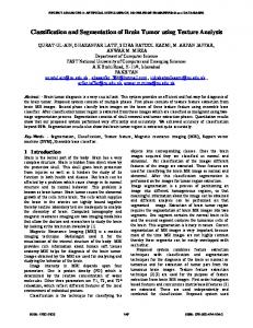
φi s(x+∆xi , y+∆yi , t+∆ti )+a(x, y, t), Figure 2. Left and Middle: two images from a 300-
i=1
(1) where the index i (1 ≤ i ≤ p) indicates the p-neighbors of the signal s(x, y, t) and a(x, y, t) is a Gaussian noise. With the noise a(x, y, t) unknown, we approximate the above formula as
frame sequence of water flowing down a dam. Right: the 3-D projection of the data points with N = 300 and l = 5. Different colors identify different groups segmented using GPCA as described later.
s(x,y,t)
£ 1 −φ1
···
¤ s(x+∆x1 ,y+∆y1 ,t+∆t1 ) −φp ≈ 0. .. . s(x+∆xp ,y+∆yp ,t+∆tp )
(2) In other words, the (p + 1)-dimensional vector [s(x, y, t), s(x + ∆x1 , y + ∆y1 , t + ∆t1 ), · · · , s(x + ∆xp , y + ∆yp , t + ∆tp )]
T
can be approximately fitted by a lower dimensional subspace (p-dimensional hyperplane). An important fact is that given a suitable choice of window size l, the signal s(x, y, t) with its p neighbors could just be entries of our N l2 -dimensional data point x(x, y). Therefore, the data points xi within the same temporal texture can be fitted by the same subspace, and since N l2 ≫ p for large enough l and N , the dimension of the subspace is much lower than N l2 .
2.2
Mixture linear models
While a single temporal texture can be modeled by a single linear model, multiple temporal textures can be better modeled using a mixture of linear models. This notion is further supported by our observation that reduceddimensional representations of data points xi obtained from sequences containing multiple temporal textures form multiple linear structures. As shown in Figure 2, the multiple linear (subspace) structure is visible in a very low dimensional projection of the data points. In Figure 2, the data points xi obtained from a video sequence of water flowing down a dam face are projected to 3-D space via principal component analysis (PCA). Instead of forming several clusters, the projected 3-D points form several linear structures. We contend that the data should be segmented from the linear structures present in the reduceddimensional representation as shown in Figure 3. Thus
2
given the data points xi ∈ RN l (i = 1, · · · , r), we first generate their low-dimensional projection yi by calculating the singular value decomposition of the matrix X = ¯ , · · · , xr − x ¯ ] such that U SV T = X with x ¯ be[x1 − x ing the average of xi (i = 1, · · · , r). Then we have the projected coordinates matrix Y = [y 1 , · · · , y r ] ∈ Rq×r such that ¯ , · · · , xr − x ¯] , Y = Sq Vq T = Uq T [x1 − x
(3)
where q is the dimension of the projection with q ≪ N l2 , Uq and Vq are the first q columns for the matrices U and V , and Sq is the first q × q block of the matrix S. As the pixel
111111 000000 000000 111111 000000 111111 000000 111111 000000 111111 000000 111111 000000 111111 000000 111111 000000 111111 000000 111111 000000 111111
1111 0000 0000 1111
Rr
Figure 3. The scheme to group the data points in low-dimensional space using mixture linear models (subspaces).
block B(x, y) around pixel s(x, y) contains both the spatial texture and temporal dynamics information around the pixel s(x, y), for textures (both spatial and temporal) with different complexity and dynamics of different orders, the corresponding linear models should have different dimensions. Therefore, given the low-dimensional representation y(x, y) for each pixel (x, y), we need to segment the y i into different low-dimensional linear models with (possibly) different dimensions.
3
Identification of the mixture linear models
3.1
with kj being the dimension of the jth subspace. Then given any data point y(x, y) it is assigned to the mth model such that
Generalized principal component analysis (GPCA)
GPCA is an algorithm for the segmentation of data into multiple linear structures [14, 13, 6]. The algorithm is non-iterative, segmentation and model identification are simultaneous. In this paper we adopt the robust GPCA algorithm, which recursively segments data into subspaces to avoid an incomplete discovery of models [6]. For example, as shown in Figure 4, data sampled from a combination of linear models may appear as though it comes from one relatively higher dimensional model e.g. the union of points on two distinct lines forms a plane.
m = arg max k DjT y(x, y) k . j
(4)
Overall, the steps for segmenting the temporal texture spatially can be summarized as following follows: (Spatial segmentation of temporal textures). Given a video sequence s, a block size l, a reduced dimension q, and an upper bound n on the system order: 1. Data sampling. Periodically sample 800-2000 pixels s(xi , yi ) and generate the corresponding N l2 dimensional data points xi . 2. Dimensionality Reduction. Compute the reduceddimensional projection of y i as the first q principal components of xi and record the projection matrix Uq . 3. Segmentation and identification of mixture linear models. Use robust GPCA to compute the segmentation of the training data y i and the bases for the linear subspaces Dj (j = 1, · · · , K).
Figure 4. The data points on the plane and the two
4. Segmentation on all pixels. For each pixel (border regions excluded) derive the data point x based on the surrounding l × l block B. Obtain its reduceddimensional representation y by projecting along Uq . Finally assign it to the mth group based on (4).
lines are first segmented as two planes and then the plane formed by the lines is further segmented into two lines. In the scenario depicted here there are two levels of recursion.
3.2
Unsupervised vs. supervised learning
4 For the segmentation problem, each pixel should be assigned to the appropriate model. This implies that for a sequence with frames sized 640×480, more than 300, 000 data points must be segmented. For current unsupervised learning algorithms, including GPCA, the computational cost would be very significant if all data points were used. In order to reduce the computational burden we turn the modeling problem from a purely unsupervised learning scenario to a hybrid scenario, i.e. we sample enough data points (in this case about 800 to 2,000 sampled either periodically or randomly) to learn the mixture of K linear models and then assign the remaining data points to the closest linear model. The sampled data is projected into qdimensional space via the maximum-variance linear trans2 formation Uq ∈ Rq×N l before applying GPCA. The K subspaces that are identified by GPCA can be described by their orthonormal basis Dj ∈ Rq×kj (j = 1, · · · , K)
Experiments and results
Water flow over dam. Figure 2 shows three images taken from a 300 frame sequence of water flow at a dam. There are multiple regions where the water dynamics are different: flow on the face of the dam, waves in the river at the bottom of the dam, and turbulence around the transition. We chose l = 5, q = 4, and used an even tiling of the sequence to produce 1,200 training data points. Applying GPCA to these low-dimensional data points, we obtained four groups as shown in Figure 5 and the model basis for each group as well. The dimensions of the four models are 3, 3, 2, and 2. Using the basis for each model, the remaining pixels were assigned according to the above algorithm to produce the segmentation shown in Figure 6. Not only does the segmentation fit our visual observation, the corresponding model dimensions also reflect the relative complexities of their textures. For the regions in
Figure 8. The four classes of pixels. The first two 20
20
40
40
60
60
80
80
100
100
120
50
100
150
120
classes belong to 7-dimensional subspaces and the last two classes belong to 6-dimensional subspaces.
50
100
150
Figure 5. Left: the mean image of the 300-frame sequence. Right: the training pixels from a 5 × 5 tiling are segmented into four classes.
Figure 9. Two sample frames from the sequence of micro-ultrasound of the mouse liver.
is clearly segmented out due to both its texture and motion due to periodic respiration. Figure 6. The four classes of pixels. groups 3 and 4 (dimension 2), the water flows with relatively simpler dynamics than in the regions of groups 1 and 2 (dimension 3) where waves are present. Trees on the river bank. Figure 7 shows three images taken from a 159-frame sequence of bushes swaying in a breeze on a river bank. The segmentation results are shown in Figure 8, the dimensions of the linear models are 7, 7, 6, and 6 respectively. While the scene is in general more complex than the previous example, the classes containing motion (classes 1 and 2) have higher dimensions than the relatively more static classes.
Figure 7. Three images from the sequence with bushes in a breeze on the river bank.
Segmentation of micro-ultrasound images. In the last example we show the results of applying our method to a 300-frame micro-ultrasound video sequence of a mouse liver. Two sample frames are shown in Figure 9. Figure 10 shows the segmentation results where the mouse’s skin
Figure 10. The four classes of pixels. In the last class, the elongated crescent structure contains the skin of the mouse.
5
Conclusion
In this paper, we proposed a novel approach for the spatial segmentation of video sequences containing multiple temporal textures. We extended the single linear model, used for homogeneous temporal textures, to a mixture linear model for scenes containing multiple temporal textures. Model identification and segmentation were implemented with a robust GPCA algorithm. A sampling process was used to identify models on a subset of the total data and the resulting models were used for complete segmentation, reducing runtime to minutes in Matlab. The effectiveness of our method was demonstrated in several examples and has applications in video synthesis and other areas including biomedical image analysis.
References [1] S. Belongie, C. Carson, H. Greenspan, and J. Malik. Color and texture-based image segmentation using em and its application to content-based image retrieval. In ICCV, pages 675–682, 1998. [2] V. Bhaskaran and K. Konstantinides. Image and Video Compression Standards: Algorithms and Architectures. Kluwer International Series in Engineering and Computer Science. Kluwer Academic Publishers, second edition, 1997. [3] M. Brand. Subspace mappings for image sequences. Technical Report TR-2002-25, Mitsubishi Electric Research Laboratory, May 2002. [4] G. Doretto, A. Chiuso, Y.N. Wu, and S. Soatto. Dynamic texture. International Journal of Computer Vision, 51(2):91–109, 2003. [5] W. Hong, J. Wright, K. Huang, and Y. Ma. Multi-scale hybrid linear models for lossy image representation. In Proceedings of the IEEE International Conference on Computer Vision, 2005. [6] K. Huang and Y. Ma. Minimum effective dimension for mixtures of subspaces: A robust gpca algorithm and its applications. In CVPR, vol. II, pages 631–638, 2004. [7] K. Huang and Y. Ma. Robust gpca algorithm with applications in video segmentation via hybrid system identification. In Proceedings of the 2004 International Symposium on Mathetmatical Theory on Network and Systems (MTNS04), 2004. [8] K. Huang, A.Y. Yang, and Y. Ma. Sparse representation of images with hybrid linear models. In ICIP, 2004. [9] B.A. Olshausen and D.J.Field. Wavelet-like receptive fields emerge from a network that learns sparse codes for natural images. Nature, 1996. [10] K. Pullen and C. Bregler. Motion capture assisted animation: Texturing and synthesis. In Proceedings of SIGGRAPH 2002, 2002. [11] M. Szummer and R.W. Picard. Temporal texture modeling. In IEEE International Conference on Image Processing, 1996. [12] M. Vetterli and J. Kovacevic. Wavelets and Subband Coding. Prentice Hall, 2000. [13] R. Vidal. Generalized principal component analysis. PhD Thesis, EECS Department, UC Berkeley, August 2003. [14] R. Vidal, Y. Ma, and S. Sastry. Generalized principal component analysis. In IEEE Conference on Computer Vision and Pattern Recognition, 2003.