Engineering, Georgia Institute of Technology, Atlanta, GA, Email: {zchen, ..... information may include routing tables, email addresses, a list of peers, and Uniform ...... between two probability mass functions p(x, t) and q(x, t) as defined in [32]:.
Spatial-Temporal Modeling of Malware Propagation in Networks Zesheng Chen, Student Member, IEEE, and Chuanyi Ji, Member, IEEE
Abstract— Network security is an important task of network management. One threat to network security is malware (malicious software) propagation. One type of malware is called topological scanning that spreads based on topology information. The focus of this work is on modeling the spread of topological malwares, which is important for understanding their potential damages, and for developing countermeasures to protect the network infrastructure. Our model is motivated by probabilistic graphs, which have been widely investigated in machine learning. We first use a graphical representation to abstract the propagation of malwares that employ different scanning methods. We then use a spatial-temporal random process to describe the statistical dependence of malware propagation in arbitrary topologies. As the spatial dependence is particularly difficult to characterize, the problem becomes how to use simple (i.e., biased) models to approximate the spatially dependent process. In particular, we propose the independent model and the Markov model as simple approximations. We conduct both theoretical analysis and extensive simulations on large networks using both real measurements and synthesized topologies to test the performance of the proposed models. Our results show that the independent model can capture temporal dependence and detailed topology information, and thus outperforms the previous models, whereas the Markov model incorporates a certain spatial dependence and thus achieves a greater accuracy in characterizing both transient and equilibrium behaviors of malware propagation. Index Terms— Security, Malware, Modeling, Stochastic processes, Graphical models
I. I NTRODUCTION Protecting a computer system from malicious attacks is a key challenge to network security and management. One such attack is due to malware propagation. The frequency and virulence of malware outbreaks have increased dramatically in the last few years, posing a significant threat to network infrastructure. Malware is malicious software in short, which is designed specially for either damaging or disrupting a computer system. This terminology is used to cover an entire gamut of hostile softwares including viruses, Trojan Horses, and network worms [1]. There are mainly two types of malwares categorized by how they spread. Active network worms such as Sapphire and Morris exploit self-propagating malicious code [2], whereas viruses such as Melissa and Concept need human interactions to spread [3]. Spreading can take place rapidly, resulting in potential network damages and service disruptions. Hence, an important step towards preventing such catastrophic events is to study the dynamic behavior of malware spreading. Zesheng Chen and Chuanyi Ji are with School of Electrical & Computer Engineering, Georgia Institute of Technology, Atlanta, GA, Email: {zchen, jic}@ece.gatech.edu. This work is supported in part by National Science Foundation under Grant ECS-0334759 and by Georgia Tech Broadband Institute 2004.
Recent investigations of malware propagation focus mostly on modeling the spread of malwares employing random scanning scheme [2], [4], [5]. Random scanning selects targets to infect randomly. Malwares, however, can use other scanning methods. For example, Morris worm exploits topological scanning, which examines local configuration files to find potential neighbors [6]. Although only a few topological malwares are known, topological scanning is a potential thread to the network routing infrastructure, World Wide Web (WWW) networks, and peer-to-peer systems [7], where topologies play an important role for malware propagation [8]. Only a handful work, however, has been done on topological-scanning malwares. For instance, contact process is used to analyze the ease of propagation on different topologies [9]. The difficulty lies in characterizing the impact of topology and the interactions among nodes in both space and time [10]. Such interactions result in a complex spatial-temporal dependence, which is especially hard to model. The goal of this work is to develop a modeling framework and mathematical models that can characterize the spread of malwares employing different scanning strategies and the impact of the underlying topology on malware propagation. To this purpose, we first abstract the problem of malware propagation using a graphical representation so that different scanning methods can be mapped to the corresponding topologies and parameters. With the help of the graphical representation, we then formulate malware propagation through a spatial-temporal random process based on the interactions among nodes. We take advantage of a discrete-time model and detailed topology information to describe the spatial and temporal statistical dependencies of malware propagation in arbitrary networks. As the temporal dependence can be naturally modeled as Markov, spatial dependence requires calculations with a multivariate probability distribution. When the number of random variables is large, an exact solution of spatial dependence is computationally too expensive to obtain. The problem then becomes how to approximate the spatial dependence using a simple, i.e., biased model, in a general setting of machine learning. In particular, spatial approximation is studied in light of the mean-field approximation [11]. Mean-field approximation is widely studied in machine learning [11] but usually for static networks where time is not involved. Exact mean-field solutions for dynamic networks are complex. Hence we consider in this work simple approximations. The simplest approximation assumes spatial independence, which is asserted in our independent model. The spatial independence assumption factorizes an exact joint probability distribution into a form that only depends on one-node marginal probabilities. Although the independent model ignores the spatial dependence, it captures temporal dependence and detailed
topology information. Simulation results show that the independent model performs better than the previous models in characterizing the transient behavior of malware propagation. A test on spatial correlation though indicates a strong spatial dependence among nodes. We therefore present the Markov model that incorporates the simplest spatial dependence as the conditional independence, motivated by the Bethe approximation used in graphical models [12]. The spatial Markov assumption factorizes an exact joint probability distribution into a form that only depends on one-node and two-node marginal probabilities. We have conducted both theoretical analysis and extensive simulations on real and synthesized topologies of large networks. Our results demonstrate that the Markov model equipped with the simple spatial dependence can achieve a greater accuracy than the independent model, especially in the sparse graphs. We then use a relative entropy to illustrate a performance gap between the Markov model and the reality, suggesting directions for further improvements. We apply our proposed models to describe the final size of infection, which corresponds to the equilibrium solution and characterizes the potential damage of malware propagation. Simulation results show that the Markov model can characterize the final size of infection no matter whether the underlying network is a homogeneous network or a complex network. Several approaches have been proposed to model and simulate malware spreading in different topologies. Kephart and White presented the Epidemiological model, which is suitable to analyze virus spreading in random graphs [10]. This work points out the difficulty in applying the Epidemiological model to study arbitrary topologies. Garetto et al. analyzed malware spreading in small-world topologies using a variation of the influence model, where the influence of neighbors is constrained to take a multilinear form [3]. Bogu˜ na ´ et al. studied epidemic spread in complex networks [13], and Wang et al. proposed a model for virus propagation in arbitrary topologies [14]. Both work [13], [14] is proposed to obtain the epidemic threshold of virus infection. Zou et al. and Wang et al. investigated the effect of topology and immunization on the propagation of computer virus through simulation [8], [15]. Ganesh et al. modeled the spread of an epidemic as a contact process [16] to study what makes an epidemic either weak or potent [9]. The model assumes that a vulnerable node can be infected by its infected neighbors at a rate that is proportional to the number of infected neighbors. Some recent investigations focus on random-scanning worms. Zou et al. modeled the spread of Code Red, taking into consideration of the human countermeasures and the worm’s impact on Internet infrastructure [4]. Chen et al. studied the propagation of active worms employing random scanning and extended the proposed modeling method to investigate the spread of localized-scanning worms [5]. Moore et al. applied the Epidemiological model to investigate the requirements for containing the self-propagation worm with random target selection [2]. The prior work, however, has not incorporated the spatial dependence on malware propagation in networks. This motivates the development of mathematical models to capture the spatial dependence, and the use of spatial models to characterize both transient and equilibrium behaviors of mal-
ware propagation with different scanning methods in arbitrary topologies. Furthermore, based on the models proposed in this paper we study the significance of the spatial dependence in determining epidemic thresholds and the speed of propagation [17]. The rest of this paper is organized as follows. In Section II, we provide a problem formulation of malware propagation. In Section III, we model the spread of malwares accurately through a spatial-temporal random process. To approximate the spatial dependence, we present the independent model and the Markov model in Sections IV and V, respectively. In Section VI, we apply our proposed models to estimate the final size of infection. We conclude this paper in Section VII with a brief summary and an outline of future work. II. M ALWARE P ROPAGATION
IN
N ETWORKS
In this section, we first introduce malware propagation briefly. We then abstract the problem using a susceptible → infected → susceptible (SIS) model and a graphical representation. Finally, we model different scanning mechanisms using graphical representations. A. Malware Propagation A computer is called infected if a malware is present there, and susceptible if it could be infected by the intrusion of the malware. If a malware cannot exist on the computer, we call this computer insusceptible to the malware. An infected computer is cured if it removes the copy of the malware and recovers to be susceptible. Final size of infection is defined as the number of initially susceptible computers that ultimately become infected in a network. The widespread occurrence of a malware is referred to as an epidemic [18]. Malware propagation is a procedure that the malware infects as many computers as possible through network connections. Those connections can be logical as to be described below. A malware can propagate in many ways. For example, when a worm is released into the Internet, it scans many machines among its neighbors in an attempt to find a susceptible machine. When a vulnerable host is found, the worm sends out a probe to infect the target. If successful, a copy of this worm is transferred to the new host, which then begins to run the worm code and tries to infect other targets. Morris worm is a typical self-propagation malware and moves from node to node using only its own and the infected node’s local information [6]. Specifically, Morris worm retrieves the neighbor list from the local Unix files /ect/hosts.equiv and /.rhosts and in individual users’ .forward and .rhosts files. Another topological worm is a SSH worm, which locates new targets by searching its current host for the names and addresses of other hosts that are likely to be susceptible to infection [19]. Email virus is an other example of topological malwares. When an email user receives an email message and opens the attachment containing a virus program, the virus infects the user’s machine and uses the recipient’s address book to send copies of itself to other email addresses. The addresses in address book represent the neighborhood relationship. A birth rate (or an infection rate) is introduced to denote the rate at which an infected computer
can infect a susceptible neighbor. The birth rate is affected by many factors. For example, for worms, the factors include the number of computer’s susceptible neighbors, payload size of the malware copy, exploited computer vulnerability, and network congestion. For email virus, the factors include email checking frequency, user vigilance in opening an email attachment, and mailbox configuration. Some malwares may have a large birth rate to flood the network as quickly as possible, whereas other malwares spread slowly and surreptitiously to evade detection and thus have a small birth rate. An infected computer might die for encountering an unexpected resource limit on the computer. Moreover, during the spreading of a malware, some infected computers may stop functioning properly, forcing the users to reboot these machines or kill some of the processes exploited by the malware. These computers are then cured, but subject to further infection. A death rate (or a cure rate) is introduced to denote the rate at which an infected computer becomes susceptible. The death rate is affected by many factors, such as resources on the computers, user alertness, the ability of a malware to disguise, and the performance of Intrusion Detection System (IDS). Combining infection and recovery, we have one of the simplest epidemiological models, the susceptible → infected → susceptible (SIS) model, which is widely used in the epidemiological research [18]. Such a model neglects the details of infection inside a single computer, abstracts the malware transmission and removal as probabilities per unit time in the form of birth rate and death rate, and considers a computer to be in one of the two possible discrete status, infected or susceptible. Although simple, the SIS model can capture key characteristics of malware spreading dynamics. The susceptible → infected (SI) model further ignores recovery and is regarded as a special case of the SIS model. The SIS model assumes that an infected computer cannot be re-infected. The model also assumes that users do not become more vigilant after experiencing a malware infection. Therefore, the birth rate and the death rate do not change with time. Moreover, in this paper we ignore patching, which is usually employed to repair security holes at the computers. This is because the spreading of malware can be much faster compared with traditional patching techniques that need human intervention, and a patch may not be available when some malware attacks unknown vulnerabilities. Nevertheless, our proposed models can be easily extended to take patching into consideration. B. Graphical Representation A malware network consists of all nodes in a network that are either infected or susceptible. A malware network can be constructed by removing insusceptible nodes and the edges associated with these nodes in the original network. Hence, a malware network is an abstraction of vulnerable nodes, which can be either end-hosts, routers, and servers, or email addresses. We use a directed graph G(V, E) to represent a malware network, where V is the set of nodes and E is the set of
S
δ7 δ2 δ3
β32
2
3 β31
β41 δ4
I
β76
6
δ6
β12
1
Fig. 1.
β72 β26
β13
4
β27
7
δ1
β65 β56 β51
5 δ5
Directed graph (S=Susceptible, I=Infected).
edges. As defined in Section II-A, each node has two status, susceptible or infected, as illustrated in Figure 1. Each edge (j, i) is associated with βji , the birth rate at which an infected node j can infect a susceptible neighbor i. Similarly, each node i is associated with δi , the death rate at which an infected node i becomes susceptible. A neighborhood of node i, denoted by Ni , is a subset of V such that every node j in this subset has an edge from node j to node i, i.e., Ni = {j|(j, i) ∈ E}. Figure 1 shows an example of directed graph wherein the neighborhood of node 1 is given as N1 = {3, 4, 5}. In this paper, we consider two widely used types of networks in the research of epidemic modeling: homogeneous networks and complex networks [13]. In a homogeneous network, each node has roughly the same nodal degree. A fully-connected topology, a standard hypercubic lattice, and an Erd¨ os-R´ enyi (ER) random network are three typical examples of homogeneous networks [20]. In a complex network, the nodal degree complies to a particular distribution. A widelystudied representative complex network has a power-law topology, where the nodal degree distribution is characterized as P (k) ∼ k −r with P (k) being the probability that a node has a degree of k [21]. It has been shown that ASlevel Internet topology, WWW networks, and some overlay topologies of peer-to-peer systems can be described by powerlaw characteristics [22], [23]. Moreover, the email groups and network exhibit the power-law distribution, which is observed in [8] and [24]. Hence, a malware network with a power-law topology can be used to study potential malware propagation on those networks. C. Scanning Methods A malware spreads by employing distinct scanning mechanisms such as random, localized, and topological scanning [7]. Although the nature of scanning methods is different, they can be modeled using the same graphical representation. Random scanning is used by some well-known malwares such as Code Red v2 and Sapphire worms. A malware that employs random scanning selects target IP addresses at random. If each IP address is visualized as a network node, random scanning results in a fully-connected topology illustrated in Figure 2(a), where the birth rate (β) is identical for every edge.
δ1
1 β δ2
2
δ1
δ6
β
6
β1
β β
β
β
β β
β
β
5
β
β
β
δ5
δ2
δ3
β
2
β2
δ3
4
δ1
6
β2 β2
β1
β2
β2
4
δ5
5 β3
δ4
3
(b) Localized Scanning.
δ5
β5
δ3
Fig. 2.
6
2
δ2
δ4
(a) Random Scanning.
δ6
β1
β2
5 β1
3
1
β1
β2
β2
β1 β
3
β2 β 1
δ6
β2
1
β4
4 δ4
(c) Topological Scanning.
Graphical representations of scanning methods.
Localized scanning is used by Code Red II and Nimda worms. Instead of selecting targets randomly, a malware preferentially scans for hosts in the “local” address space. Such a scanning scheme results in a fully-connected topology such as the one illustrated in Figure 2(b), where nodes within a group (e.g., IP addresses with the same first two octets) infect one another with the same birth rate (β1 ), whereas nodes in different groups infect one another with a different birth rate (β2 ). Topological scanning is used by Email viruses and Morris/SSH worms. The malware relies on the information contained in the victim machine in order to locate new targets. The information may include routing tables, email addresses, a list of peers, and Uniform Resource Locations (URLs). Topological scanning scheme can result in an arbitrary topology such as an undirected power-law topology illustrated in Figure 2(c), where βi ’s and δi ’s (i = 1, 2, · · · , 5) represent different birth rates and death rates. Although only a few topological worms are known, topological scanning is worth investigating for the following reasons. First, the network routing infrastructure, World Wide Web (WWW) networks, and peer-to-peer systems are vulnerable to topological scanning. For example, a malware attacking a website could look for neighboring websites in its URLs and use these websites as targets. Second, when IPv4 is upgraded to IPv6, the address space will be much sparser. It would be difficult for either random-scanning or localized-scanning worms to find a target in the IPv6 address space. Therefore, topological scanning may be preferred by attackers. Finally, models of such malware-propagation would provide insights for developments of countermeasures, which are lacking for topological worms. III. S PATIAL - TEMPORAL M ODEL The problem of modeling malware propagation in networks can be stated as follows: Given a malware network topology, values of βji ’s and δi ’s, and an initial infection node, what is the expected number of infected nodes at time t? To approach this problem, we formulate malware propagation through a spatial-temporal random process based on local interactions of nodes in networks. Let Xi (t) denote the status of a network node i at time t,
β i (t) 1−β i (t)
S
I
1− δ i
δi Fig. 3.
State diagram of a node i.
where t represents discrete time. � 1, if node i is infected at time t; Xi (t) = 0, if node i is susceptible at time t. As node i can be infected only by its neighbors, Xi (t) is statistically dependent on Xi (t − 1) and the status of its neighbors. Since the status of a neighbor also depends on its own neighbors, conceptually, the status of all nodes is statistically dependent in space and time. Let vector X(t) denote the status of all nodes at time t, i.e., X(t) = {X1 (t), X2 (t), · · · , XM (t)}, where M represents the total number of nodes in the network. X(t) is then a spatialtemporal process. If node i is susceptible, it can be compromised by any of its infected neighbors, e.g., node j, with a birth rate βji . Therefore, given the status of the neighbors of node i, at the next time step the susceptible node i can get infected with Q probability βi (t) = 1− j∈Ni (1−βji )xj (t) , where xj (t) is the realization of the status of node j at time t and xj (t) = 0 or 1. Otherwise, node i is infected and has a death rate δi to recover at the next time step. This procedure can be expressed by a Markov chain in Figure 3. Therefore, the temporal dependence of node i can be shown as: P (Xi (t + 1) = 0|Xi (t) = 1) = δi , P (Xi (t + 1) = 1|Xi (t) = 0, XNi (t) = xNi (t)) = βi (t),
(1) (2)
where vector XNi (t) is used to denote the status of all neighbors of node i at time t and vector xNi (t) is the realization of XNi (t), i.e., XNi (t) = {Xj (t), j ∈ Ni } and xNi (t) = {xj (t), j ∈ Ni }. If for ∀j, βji 0 (or ρij < 0). We obtain the correlation coefficients through simulation on a four-neighbor 2D-lattice, with 10,000 nodes, β = 0.1, δ = 0.1, and 1,000 individual runs. In this 2D-lattice, each node is
represented by its coordinate (x, y), where x, y are integers and 0 ≤ x, y ≤ 99. Node (x, y) has four neighbors (x − 1, y), (x + 1, y), (x, y − 1), and (x, y + 1), where the arithmetic operations are modular on 100. We assume that the malware begins to spread from node (0, 0), and consider the correlation coefficients between the status of node (0, 0) and node (0, i) (denoted by ρi (t)) for i = 1, 2, 3. Figure 7 shows how the correlation coefficients vary with time. It is observed that the correlation coefficients are initially close to 0, but increase with time. When t > 50, all coefficients are larger than 0.25. This shows a strong dependence in space among nodes, and suggests a better model that accounts for spatial dependence. V. M ARKOV M ODEL A. Model Our Markov model assumes a conditional independence in space [28]. That is, at time t (t = 1, 2, 3, · · · ), given the status of node i the status of its neighbors is (conditionally) independent, P (XNi (t) = xNi (t)|Xi (t) = xi (t)) Y = P (Xj (t) = xj (t)|Xi (t) = xi (t)).
(16)
j∈Ni
With the spatial Markov assumption, the dependency graph shown in Figure 4(a) is changed to the graph shown in Figure 4(c), where the edges between the neighbors of node i are deleted. The spatial Markov assumption is motivated by the Bethe approximation [12], a way of deriving and correcting the mean-field theory, which has been widely investigated in the area of machine learning. The Bethe approximation factorizes an exact joint probability distribution into a form that only depends on one-node and two-node marginal probabilities in a Markov network. Moreover, the Bethe approximation is shown to be equivalent to belief propagation in [12]. Here we adopt the spirit of the Bethe approximation by incorporating a simple spatial dependence into the Markov model. Theorem 2: (Markov Model) If the status of node i’s neighbors at the same time step is spatially independent given the status of node i, then the state evolution of node i from Equation (5) satisfies P (Xi (t + 1) = 1) = 1 − Ri (t) − P (Xi (t) = 0)Simar (t),
(17)
where Simar (t) =
Y
(18)
[1 − βji P (Xj (t) = 1|Xi (t) = 0)].
j∈Ni
P ROOF: Since the status of node i’s neighbors at time t is spatially independent given the status of node i, as shown by Equation (16), Equation (4) yields Simar (t) i X Y h = P (Xj (t) = xj (t)|Xi (t) = 0)(1 − βji )xj (t) xNi (t) j∈Ni
=
Y Xh
P (Xj (t) = xj (t)|Xi (t) = 0)(1 − βji )xj (t)
j∈Ni xj (t)
=
Y
j∈Ni
[1 − βji P (Xj (t) = 1|Xi (t) = 0)] .
i
The computation of the conditional probability P (Xj (t) = 1|Xi (t) = 0) is given in the Appendix. The Markov model takes into account a part of the neglected correlations between random variables (i.e., node i and its neighbors at time t) and thus improves the approximation. The Markov model differs from the independent model only in the probability that one of node i’s neighbors infects node i. This probability is βji P (Xj (t) = 1|Xi (t) = 0) for the Markov model, whereas it is βji P (Xj (t) = 1) for the independent model. If the dependence between node i and its neighbors is ignored, the Markov model is reduced to the independent model. Moreover, with the spatial Markov assumption, if node i has k neighbors, the total number of status needed to describe the joint probability P (XNi (t) = xNi (t)|Xi (t) = 0) is O(k). Is it always beneficial to incorporate the spatial dependence? We investigate this issue by introducing the notion of association defined in [29]. Definition 1: Random variables T1 , · · · , Tn are associated if Cov[f (T), g(T)] = E[f (T)g(T)] − E[f (T)]E[g(T)] ≥ 0
for all nondecreasing functions f and g for which E[f (T)], E[g(T)], and E[f (T)g(T)] exist, and T = {T1 , · · · , Tn }. In most cases, if one neighbor of node i, e.g., node j, is infected, node i then has an increasing probability to be infected. That is, node i and node j are positively correlated as shown in Figure 7. Therefore, the status of nodes i and j, Xi (t) and Xj (t), is associated by definition. Furthermore, if Xi (t) and XNi (t) are associated random variables, we can show in the following theorem that the Markov model indeed achieves better performance than the independent model. Theorem 3: (Performance Bound) If Xi (t) and XNi (t) are associated, then Siind (t) ≤ Simar (t) ≤ Si (t). (19) P ROOF: Since Xi (t) and Xj (t) (j ∈ Ni ) are associated, Cov[Xi (t), Xj (t)] ≥ 0. We can write P (Xi (t) = 1, Xj (t) = 1) ≥ P (Xi (t) = 1) · P (Xj (t) = 1),
which leads to P (Xj (t) = 1) ≥ P (Xj (t) = 1|Xi (t) = 0).
(20)
Therefore, Siind (t) ≤ Simar (t). Given Xi (t) Q = 0, let f (XNi (t)) = −(1 − βli )Xl (t) and g(XNi (t)) = − j∈Ni −{l} (1−βji )Xj (t) , where l ∈ Ni . Since XNi (t) are associated, from the definition of association we have Cov [f (XNi (t)), g(XNi (t))|Xi (t) = 0] ≥ 0,
(21)
which leads to E [f (XNi (t))|Xi (t) = 0] · E [g(XNi (t))|Xi (t) = 0] ≤ E [f (XNi (t))g(XNi (t))|Xi (t) = 0] .
Repeated use of the above argument yields Y
h i E (1 − βji )Xj (t) |Xi (t) = 0
j∈Ni
2
≤ E4
Y
j∈Ni
3
(1 − βji )Xj (t) |Xi (t) = 05 .
That is, Simar ≤ Si (t).
(22)
Independent (β=0.5) Markov (β=0.5) Simulation (β=0.5) Independent (β=0.1) Markov (β=0.1) Simulation (β=0.1) Independent (β=0.05) Markov (β=0.05) Simulation (β=0.05)
10
5
14
4
x 10
12 10 8
14
Independent (δ=0.05) Markov (δ=0.05) Simulation (δ=0.05) Independent (δ=0.1) Markov (δ=0.1) Simulation (δ=0.1) Independent (δ=0.2) Markov (δ=0.2) Simulation (δ=0.2)
6 4 2
0 0
1000
2000
3000 time
4000
5000
6000
(a) A 2D-lattice with 160,000 nodes and δ = 0.1.
0 0
Independent (=6) Markov (=6) Simulation (=6) Independent (=4) Markov (=4) Simulation (=4) Independent (=2) Markov (=2) Simulation (=2)
10 8 6 4 2
20
40
time
60
80
100
(b) An ER random graph with 160,000 nodes, k = 4, and β = 0.1. Fig. 8.
4
x 10
12
number of infected nodes
4
x 10
number of infected nodes
number of infected nodes
15
0 0
50
100
150 time
200
250
300
(c) A BA network with 160,000 nodes, β = 0.1, and δ = 0.1.
Malware propagation in different topologies.
B. Performance How much does the spatial Markov dependence help in improving the performance? We compare the performance of our proposed models with the simulation results in 2D-lattice, ER random graph, BA power-law network, a real topology, and a top-down hierarchical topology. Except for the 2Dlattice, which is a regular graph, we begin each simulation and models with a single, randomly chosen infected node on a given topology. Each plot considers 10 different initiallyinfected nodes, and each simulation plot also has 10 individual runs for an initially-infected node. Figure 8(a) compares the performance of the independent model and the Markov model with the simulation results on a four-neighbor 2D-lattice. The number of nodes M = 160, 000 and the death rate δ = 0.1. For the case of the birth rate β = 0.5, the three curves nearly coincide with each other. When β decreases, however, the infection spreads at a faster rate in both the independent and the Markov models than the simulation. In all three cases (β = 0.5, β = 0.1, β = 0.05), the Markov model yields more accurate results than the independent model. Figure 8(b) shows the predictions of two models with the simulation results on an ER random graph, with 160,000 nodes, an average nodal degree k = 4, and β = 0.1. When we constructed the ER random graph, the generated graph was disconnected for that k is small. Therefore, in this disconnected graph we chose the largest cluster with 156,763 nodes and an average degree of 4.07 as the target network. It can be seen that the Markov model yields far better performance than the independent model when compared with the simulation results. Figure 8(c) depicts the simulation results against two models on a BA network, with 160,000 nodes, β = 0.1, δ = 0.1, and < k >= k. For the case when k = 6, both models give precise results. When k decreases, however, the predictions of both models become worse. In all three cases (k = 6, k = 4, k = 2), the Markov model predicts malware propagation more accurately than the independent model. It is observed that the parameters can affect the accuracy of
the models. When β or k is large, both the independent model and the Markov model perform well. When both β and k are small, however, both models fail to predict the slow growth of malware propagation. Therefore, both models are suited for dense graphs, where each node fluctuates independently about its mean value. On the other hand, the Markov model outperforms the independent model in all cases with different parameters and underlying topologies. That is, Theorem 3 is confirmed by the results shown in Figure 8. Another observation is that the underlying topology can affect the speed of malware propagation and the final size of infection. For the case of β = 0.1 and δ = 0.1, although all three graphs (Figure 8) have the same number of nodes and edges, the malware spreading dynamics in these graphs are significantly different. It takes the malware about 1,716 time steps to enter an equilibrium stage in the 2D-lattice, whereas it needs about 100 time steps and 66 time steps in the ER random graph and the BA network, respectively. Moreover, after entering the equilibrium stage, the malware infects a total of 112,506 nodes in the 2D-lattice, 106,023 nodes in the ER random graph, and 105,511 nodes in the BA network. This shows the effect of network structure on the dynamics of malware propagation. Figure 9 shows malware propagation in real topology, ER random graph, BA network, and four-neighbor 2D-lattice for the special case when β = 1 and δ = 0.1. The real topology is an AS graph collected at the Oregon router server routeviews.oregon-ix.net, which is a site for collecting BGP data [30]. The dataset is selected on 1 June 2004 and contains 38,086 links among 17,653 ASes (k = 4.3). The constructed ER random graph has a largest cluster with 17,648 nodes and k = 4.3, and the malware only propagates in this largest cluster. The BA network has 17,652 links among 17,653 nodes (k = 2). The generated BA network is connected and thus is a tree. The 2D-lattice is with 17,689 nodes and k = 4. Among all these four topologies, the curves of both models overlap with the simulation results in this special case. Therefore, both models can achieve the best performance in the case of β = 1. Although the AS graph and the ER random graph have
1.4
18000 16000
Independent model (D(p||q1)) Markov model (D(p||q2))
1.2 1
12000 10000
Relative Entropy
number of infected nodes
14000
Independent (Oregon) Markov (Oregon) Simulation (Oregon) Independent (Random) Markov (Random) Simulation (Random) Independent (BA) Markov (BA) Simulation (BA) Independent (Lattice) Markov (Lattice) Simulation (Lattice)
8000 6000 4000 2000 0 0
50
time
100
0.2 150
50
100
150
200
250
Fig. 11. Relative entropies in 2D-lattice with 10,000 nodes, β = 0.1, and δ = 0.1.
4
C. Test of Spatial Markov Assumption
12
number of infected nodes
0 0
time
x 10
10 8 Independent (β=0.02) Markov (β=0.02) Simulation (β=0.02) Independent (β=0.01) Markov (β=0.01) Simulation (β=0.01) Independent (β=0.005) Markov (β=0.005) Simulation (β=0.005)
6 4 2 0 0
0.6 0.4
Fig. 9. Malware propagation in real topology, ER random graph, BA network, and 2D-lattice with β = 1 and δ = 0.1.
14
0.8
500
1000 time
1500
2000
Fig. 10. Malware propagation in a top-down hierarchical topology with 129,480 nodes, 266,005 edges, and δ = 0.
almost the same number of (connected) nodes and average nodal degree, the malware takes only 6 time steps to enter an equilibrium stage in the AS graph, whereas it needs about 9 time steps in the ER random graph. This shows that these two topologies have different diameters and the AS graph is more vulnerable to malware propagation than the ER random graph. It is interesting to notice that although the dynamics of malware spreading in different topologies are distinct, the final sizes of infection are almost the same, i.e., n(t) ≈ 16, 000, when t = 150. This reflects that for the case when β = 1 and δ = 0.1, the final size of infection is not dependent on the network structure, but on the total number of nodes. Figure 10 demonstrates another special case when δ = 0, which corresponds to the susceptible → infected (SI) model. The malware spreads in a top-down hierarchical topology generated by BRITE [26]. The top AS-level topology is from NLANR on 2 January 2000 [31], with 6,474 ASes and 13,895 interconnections. The down router-level topology is generated by BRITE router-level BA model, with 20 nodes per AS. The constructed top-down hierarchical topology has 129,480 nodes and 266,005 edges. The merit of the Markov model can also be observed in this special case when δ = 0.
To further examine the goodness of spatial Markov assumption, we use a relative entropy (or Kullback-Leibler distance) between two probability mass functions p(x, t) and q(x, t) as defined in [32]: X p(x, t) p(x, t)log D(pkq) = . (23) q(x, t) x The relative entropy is a measure of the distance between two distributions p(x, t) and q(x, t). If q(x, t) is “closer” to p(x, t), D(pkq) is smaller; and D(pkq) = 0 if and only if p = q. For our case, p(x, t) = P (XNi (t) = xNi (t)|Xi (t) = 0) is the joint distribution of the status of node i’s neighbors given node i is susceptible at time t. For the independent Q model, q1 (x, t) = Qj∈Ni P (Xj (t) = xj (t)); for the Markov model, q2 (x, t) = j∈Ni P (Xj (t) = xj (t)|Xi (t) = 0). We obtain the relative entropies D(pkq1 ) and D(pkq2 ) through simulation on a four-neighbor 2D-lattice, with 10,000 nodes, β = 0.1, δ = 0.1, and 1,000 individual runs. As described in Section IV-C, each node is represented by its coordinate and the malware begins to spread from node (0, 0). Node i is specified at (1, 1). Figure 11 shows how the relative entropies D(pkq1 ) and D(pkq2 ) change with time. It is observed that the relative entropies are initially close to 0, but increase with time. D(pkq2 ) is smaller than D(pkq1 ) for all time t, suggesting that the spatial Markov model is indeed a better approximation than the spatial independent model. On the other hand, when t > 60, D(pkq2 ) > 0.5. This explains the performance gap between the Markov model and the simulation observed in Figures 8 and 10. Hence, a model that incorporates more spatial dependence than the Markov model may result in a smaller relative entropy. VI. F INAL S IZE
OF I NFECTION
The final size of infection corresponds to the equilibrium state of a malware network, which is the average number of infected nodes when time t approaches infinity, i.e., limt→+∞ n(t). The final size of infection characterizes the potential damage due to malware propagation. If the final size
10000
9000
9000
8000
8000
7000
7000
final size of infection
final size of infection
10000
6000 5000 4000 3000 Simulation Epidemiological model AAWP model Independent model Markov model
2000 1000 0 −3 10
−2
10
−1
birth rate
10
5000 4000 3000 2000 1000
0
10
(a) An ER random graph with 10,000 nodes, k = 10, and δ = 0.1. Fig. 12.
6000
0 −3 10
Simulation UCN model Independent model Markov model −2
10
−1
death rate
10
0
10
(b) A BA network with 10,000 nodes, k = 4, and β = 0.1.
Performance comparisons in estimating the final size of infection.
of infection can be predicted at an early stage of malware spreading, the potential damage can be assessed and preventive actions can be taken accordingly. In this section, we compare our proposed models with the simulation results and the other models in estimating the final size of infection in homogeneous and complex networks. Each simulation scenario has 100 individual runs and is averaged over the cases that the malware survives. The final size of infection is sampled at time t = 2000. Figure 12(a) shows a comparison of the Epidemiological model, the AAWP model, the independent model, the Markov model, and the simulation results on a connected ER random graph, with 10,000 nodes, k = 10, and δ = 0.1. When compared with the simulation results, the Epidemiological model over-predicts the final size of infection when β ≥ 0.02, whereas the AAWP model and the independent model slightly over-predict it. The results of the Markov model and the simulation overlap for 0.001 ≤ β ≤ 1. Therefore, the Markov model is the most accurate one among all these models. Figure 12(b) gives another comparison of the UCN model, the independent model, the Markov model, and the simulation results on a BA network, with 10,000 nodes, k = 4, and β = 0.1. The UCN model over-predicts the final size of infection, whereas the independent model slightly over-predicts it. The results of the Markov model and the simulation overlap for 0.001 ≤ δ ≤ 1. Therefore, both the independent model and the Markov model are shown to be good estimators of the final size of infection, and the Markov model is more accurate than the independent model. VII. C ONCLUSIONS In this paper, we have presented a spatial-temporal model to study the dynamic spreading of malwares that employ different scanning methods. Making use of this model, we have studied the impact of the underlying topology on malware propagation. We show that detailed topology information and spatial dependence are key factors in modeling the spread of malwares. The
independent model incorporates detailed topology information and thus outperforms the previous models. Our Markov model incorporates both detailed topology information and simple spatial dependence, and thus achieves a greater accuracy than the independent model, especially when both the birth rate and the average nodal degree are small. Moreover, when the graph is dense, each node fluctuates independently about its mean value and thus both models perform well. These results are validated through analysis and extensive simulations on large networks using real and synthesized topologies. The class of models we have investigated are biased, i.e., with a reduced complexity. Hence, the performance of such models is important. Relative entropy is used as a performance measure and shows that a performance gap still exists between the Markov model and the reality. Formulations are needed to incorporate more spatial dependence into the model. Furthermore, as both models are motivated by the spirit of the mean-field approximation in machine learning, a formal treatment of the mean-field approximation to include temporal dependence will be studied in our future work. As part of the ongoing work, we also plan to estimate the parameters of malware propagation (e.g., birth rate and death rate) and use our proposed models to study the countermeasures for controlling the spread of malwares. Our modeling approach may also help to understand a wide range of information propagation behavior in Internet, such as BGP update streams and file sharing in peer-to-peer applications. ACKNOWLEDGEMENTS The authors would like to thank Dr. Mostafa H. Ammar, Guanglei Liu, and Rajesh Narasimha at Georgia Tech for many useful discussions, and thank Dr. Cliff C. Zou for pointing out the errors in Equations (13) and (14). The authors would also like to thank the anonymous reviewers for their valuable comments.
R EFERENCES [1] Richard Ford, “Malware website,” http://www.malware.org/malware.htm. [2] D. Moore, C. Shannon, G. M. Voelker, and S. Savage, “Internet Quarantine: Requirements for Containing Self-Propagating Code,” in Proc. of INFOCOM 2003, San Francisco, April 2003. [3] M. Garetto, W. Gong, and D. Towsley, “Modeling Malware Spreading Dynamics,” in Proc. of INFOCOM 2003, San Francisco, April 2003. [4] C. C. Zou, W. Gong, and D. Towsley, “Code Red Worm Propagation Modeling and Analysis,” in 9th ACM Conf. on Computer and Communication Security, Washington DC, Nov. 2002. [5] Z. Chen, L. Gao, and K. Kwiat, “Modeling the Spread of Active Worms,” in Proc. of INFOCOM 2003, San Francisco, April 2003. [6] H. Orman, “The Morris worm: a fifteen-year perspective,” IEEE Security & Privacy Magazine, vol. 1, pp. 35–43, Sept./Oct. 2003. [7] S. Staniford, V. Paxson, and N. Weaver, “How to 0wn the Internet in Your Spare Time,” in Proc. of the 11th USENIX Security Symposium (Security ’02), 2002. [8] C. C. Zou, D. Towsley, and W. Gong, “Email Worm Modeling and Defense,” in 13th International Conf. on Computer Communications and Networks, Chicago, Oct. 2004. [9] A. Ganesh, L. Massoulie, and D. Towsley, “The Effect of Network Topology on the Spread of Epidemics,” in Proc. of INFOCOM 2005, Miami, March 2005. [10] J. O. Kephart and S. R. White, “Directed-Graph Epidemiological Models of Computer Viruses,” in Proc. of the 1991 IEEE Computer Society Symposium on Research in Security and Privacy, 1991, pp. 343–359. [11] M. Opper and D. Saad (Eds.), “Advanced Mean Field Methods, Theory and Practice,” MIT Press, Feb. 2001. [12] J. S. Yedidia, “An Idiosyncratic Journey Beyond Mean Field Theory,” Advanced Mean Field Methods, Theory and Practice, pp. 21–36, Feb. 2001. [13] M. Bogu˜ na ´ , R. Pastor-Satorras, and A. Vespignani, “Epidemic spreading in complex networks with degree correlations,” in “Statistical Mechanics of Complex Networks”, eds. R. Pastor-Satorras et al., Lecture Notes in Physics 625, 2003, pp. 127–147. [14] Y. Wang, D. Chakrabarti, C. Wang, and C. Faloutsos, “Epidemic Spreading: An Eigenvalue Viewpoint,” in Proc. of the 2003 Symposium of Reliable and Distributed Systems, Florence, Italy, Oct. 2003. [15] C. Wang, J.C. Knight, and M. Elder, “On Viral Propagation and the Effect of Immunization,” in 16th ACM Annual Computer Applications Conference, New Orleans, Dec. 2000. [16] T. M. Liggett, “Interacting Particle Systems,” Springer, 1985. [17] R. Narasimha, C. Ji, and Z. Chen, “Understanding the Significance of Spatial Dependence in Modeling Malware Propagation on Networks,” submitted to IEEE Transaction on Signal Processing, 2005. [18] H. Andersson and T. Britton, “Stochastic Epidemic Models and Their Statistical Analysis,” in Lecture Notes in Statistics, Springer-Verlag, 2000, vol. 151. [19] S. E. Schechter and J. Jung, “Inoculating SSH Against AddressHarvesting Worms,” http://nms.csail.mit.edu/projects/ssh/. [20] P. Erd¨ os and A. R´ enyi, “On the evolution of random graphs,” in Publ. Math. Inst. Hung. Acad. Sci., 1960, vol. 5, pp. 17–61. [21] M. Faloutsos, P. Faloutsos, and C. Faloutsos, “On Power-Law Relationships of the Internet Topology,” in Proc. of ACM SIGCOMM 1999, 1999, pp. 251–262. [22] A. Barab´ a si and R. Albert, “Emergence of scaling in random networks,” in Science 286, 1999, pp. 509–512. [23] S. Saroiu, P. K. Gummadi, and S. D. Gribble, “A Measurement Study of Peer-to-Peer File Sharing Systems,” in Proc. of Multimedia Computing and Networking 2002 (MMCN’02), Jan. 2002. [24] H. Ebel, L. Mielsch, and S. Bornholdt, “Scale-free topology of e-mail networks,” in Phys. Rev. E 66, 035103(R), 2002. [25] M. J. Wainwright and M. I. Jordan, “Graphical models, exponential families, and variational inference,” Tech. Rep. Technical Report 649, Department of Statistics, University of California, Berkeley, 2003. [26] A. Medina, A. Lakhina, I. Matta, and J. Byers, “BRITE: Universal Topology Generation from a User’s Perspective,” Tech. Rep. (User Manual) BU-CS-TR-2001-003, April 2001. [27] A. V´ azquez, R. Pastor-Satorras, and A. Vespignani, “Large-scale topological and dynamical properties of the Internet,” in Physical Review E 65, 066130, 2002. [28] S. L. Lauritzen, “Graphical Models,” Oxford University Press Inc., 1996.
[29] J. D. Esary, F. Proschan, and D. W. Walkup, “Association of Random Variables, with Applications,” in The Annals of Mathematical Statistics, Oct. 1967, vol. 38, pp. 1466–1474. [30] University of Oregon Advanced Network Technology Center, “University of Oregon Route Views Project,” http://routeviews.org/. [31] Measurement National Laboratory for Applied Network Research and Network Analysis Group (NLANR/MNA), “NLANR Routing Raw Data,” http://moat.nlanr.net/Routing/rawdata. [32] T. M. Cover and J. A. Thomas, “Elements of Information Theory,” John Wiley & Sons, 1991.
APPENDIX Computation of Conditional Probability To calculate the conditional probability P (Xj (t) = 1|Xi (t) = 0), we introduce a two-node joint probability P (Xi (t) = 1, Xj (t) = 1). Thus, P (Xj (t) = 1|Xi (t) = 0) P (Xj (t) = 1) − P (Xi (t) = 1, Xj (t) = 1) = . P (Xi (t) = 0)
(24)
To simply the notation, we set Puv (t) = P (Xi (t + 1) = 1, Xj (t + 1) = 1|Xi (t) = u, Xj (t) = v), where u, v ∈ {0, 1}. The two-node joint probability can be obtained by the following equations: P (Xi (t + 1) = 1, Xj (t + 1) = 1) X = [P (Xi (t) = u, Xj (t) = v)Puv (t)] ,
(25)
u,v
where the total probability theorem is used and P11 (t) = (1 − δi )(1 − δj ),
(26)
since given that both node i and node j are infected at time t, they independently choose to stay in infected status; P01 (t) = (1 − δj )[1 − Si0 (t)], in that thus
Si0 (t)
(27)
= P (Xi (t + 1) = 0|Xi (t) = 0, Xj (t) = 1) and Y
Si0 (t) = (1 − βji )
[1 − βli P (Xl (t) = 1|Xi (t) = 0)],
l∈Ni −{j}
where the spatial Markov assumption is used; similarly, P10 (t) = (1 − δi )[1 − Sj0 (t)],
(28)
in that Sj0 (t) = (1 − βij )
Y
[1 − βlj P (Xl (t) = 1|Xj (t) = 0)];
l∈Nj −{i}
P00 (t) ≈ [1 − Si00 (t)][1 − Sj00 (t)],
(29)
where Si00 (t) =
Y
[1 − βli P (Xl (t) = 1|Xi (t) = 0)],
Y
[1 − βlj P (Xl (t) = 1|Xj (t) = 0)].
l∈Ni −{j}
Sj00 (t) =
l∈Nj −{i}
Equation (29) uses an approximation to avoid the introduction of a three-node joint probability P (Xi (t) = 0, Xj (t) = 0, Xl (t) = xl (t)) if nodes i, j, l construct a triangle. Equation (25) is obtained by replacing Puv (t) with the results from Equations (26) ∼ (29). Equations (17) and (25) provide a recursive relationship between Xi (t + 1), Xj (t + 1) and Xi (t), Xj (t) for j ∈ Ni . It is assumed that the status of all nodes is independent at time 0.