Spatialising crop models - HAL-Inria

Spatialising crop models Robert Faivre, Delphine Leenhardt, Marc Voltz, Marc Benoˆıt, Fran¸cois Papy, G´erard Dedieu, Daniel Wallach

To cite this version: Robert Faivre, Delphine Leenhardt, Marc Voltz, Marc Benoˆıt, Fran¸cois Papy, et al.. Spatialising crop models. Agronomie, EDP Sciences, 2004, 24 (4), pp.205-217. .

HAL Id: hal-00886026 https://hal.archives-ouvertes.fr/hal-00886026 Submitted on 1 Jan 2004

HAL is a multi-disciplinary open access archive for the deposit and dissemination of scientific research documents, whether they are published or not. The documents may come from teaching and research institutions in France or abroad, or from public or private research centers.

L’archive ouverte pluridisciplinaire HAL, est destin´ee au d´epˆot et `a la diffusion de documents scientifiques de niveau recherche, publi´es ou non, ´emanant des ´etablissements d’enseignement et de recherche fran¸cais ou ´etrangers, des laboratoires publics ou priv´es.

205

Agronomie 24 (2004) 205–217 © INRA, EDP Sciences, 2004 DOI: 10.1051/agro:2004016

Review article

Spatialising crop models Robert FAIVREa, Delphine LEENHARDTb*, Marc VOLTZc, Marc BENOÎTd, François PAPYe, Gérard DEDIEUf, Daniel WALLACHb a Institut National de la Recherche Agronomique, Unité BIA, BP 27, 31326 Castanet Tolosan Cedex, France Institut National de la Recherche Agronomique, UMR ARCHE, BP 27, 31326 Castanet Tolosan Cedex, France c Institut National de la Recherche Agronomique, UMR LISAH, Bât. 24, place Viala, 34060 Montpellier Cedex 1, France d Institut National de la Recherche Agronomique, UR SAD, BP 29, 88501 Mirecourt, France e Institut National de la Recherche Agronomique, UR SAD, BP 01, 78850 Thiverval-Grignon, France f Centre National d’Études Spatiales, CESBIO UMR 5126, 18 avenue Edouard Belin, 31401 Toulouse Cedex 9, France b

(Received 12 June 2003; accepted 26 March 2004)

Abstract – There are many incentives for applying a crop model on a regional scale, i.e. over an area larger than that for which it has been developed. This is what we call “spatialising” a crop model. These large areas can have very heterogeneous soil, climate and management practices. Consequently, spatialising a crop model can raise serious problems. One set arises from the fact that the basic concepts, hypotheses and validity domains of crop models are derived on the plot scale and may not apply on a larger scale. Another set arises from the lack of adequate and sufficient data to run the model on a regional scale. The workshop held in Toulouse (France) on 14–15 January 2002 dealt with the topic of spatialising crop models. The present paper is a comprehensive summary of the thoughts we had before, during and after the workshop. crop modelling / scale change / spatial variability

1. INTRODUCTION The recent development of genetically modified organisms (GMO), the new European Water Directive (2000) emphasising water quality, or climatic change and its impact on crop development, runoff and irrigation demand raise new scientific issues. The answers require in many cases the application of crop models on a regional scale, with concomitant large heterogeneities in soil, climate and management practices between fields. Using a crop model over areas larger than those over which it was developed is what we will call “spatialising the crop model”. When all the information needed by the model (input data and parameters) is available, this can be done quite easily from a computational point of view but it still raises questions that need to be answered. Some of them arise from the fact that the basic concepts, hypotheses and validity domains of crop models were derived on the plot scale and are too restrictive when applying the models on larger scales. Others arise from the lack of adequate and sufficient data to run the model on regional scales. To clarify and attempt to answer these questions, a workshop was held in Toulouse (France) on 14–15 Jan-

* Corresponding author: [email protected]

uary 2002 on the topic of spatialising crop models. The authors of the present paper are the scientific organisers of the workshop and the sessions' chairmen. The present paper is a comprehensive summary of the thoughts we had before, during and after the workshop. In particular, it is based on a summary of concluding notes taken by the various session chairmen at the end of the workshop. The analysis in terms of scale change arose from discussions held during the workshop, and continued after the workshop in a summer school entitled “for a good use of crop models” and organised by INRA in Le Croisic (France) on 14–18 October 2002. In the next section, we first describe the main characteristics of crop models and we define what we call the scale of a crop model, pointing out in examples some specific questions that have to be answered before spatialising a crop model. In the third section, we summarise some spatialisation techniques that were presented during the workshop or in the literature. A presentation using the viewpoint of scale change is presented in the fourth section, before discussing alternative approaches as a conclusion to the paper.

206

R. Faivre et al.

2. CROP MODEL AND SCALE 2.1. Main characteristics of crop models Crop models are mathematical representations of the soilplant-atmosphere system (SPA system), involving interactions between biological factors and environment [24]. They calculate crop growth and yield, as well as the soil and plant water and nutrient balances, as a function of environmental conditions and crop management practices. The equations used in crop models represent the elementary processes of the SPA system. Three main modules or processes can therefore be identified. The soil module represents water transfer within the soil, which includes infiltration, drainage and redistribution [34]. The infiltration of water into the soil derives from the input of water, mainly by rainfall or irrigation, and results in a heterogeneous distribution of water in the soil profile. The soil module can also represent nutrient transfer, and specifically nitrogen transport and transformations [8]. The plant module describes two mechanisms: (i) the growth of the canopy, i.e. the production of biomass, based on interception and transformation of the photosynthetically active radiation and modulated by senescence, and (ii) the development of the crop, that simulates the main stages of crop life (germination, flowering, production of seeds and senescence) and drives growth by organising, throughout development, the opening and closing of sinks, and by acting on sources [7]. The atmosphere module links the soil and plant modules. It represents evapotranspiration, which corresponds to two processes: (i) the evaporation from the soil and (ii) plant transpiration or root extraction. These two processes can be simulated as a whole or separately. It allows interactions between the plant and the soil module: when water supply in the soil becomes limiting, the main physiological processes such as photosynthesis and leaf expansion are reduced, depending on the intensity of the stress. Infiltration, drainage, redistribution and evapotranspiration are generally assumed to be one-dimensional and vertical. Mathematically speaking, crop models consist of a series of equations, f. These equations contain parameters (or internal coefficients), θ, which, once the model has been calibrated, remain unchanged from one simulation to another. The models work with input data, v, variable in time (including weather data such as precipitation and temperature, and management practices such as dates and quantities of irrigation or fertilisation), or fixed, specific to the simulated crop (soil characteristics of the plot in question: soil type, soil depth, cultivar or variety, etc.). They output variables, y (yield, evolution of leaf area index or dry matter, water requirements, leached nitrate, etc.). One can thus adopt the following notation: y = f(θ, v). The parameters θ of a crop model can be numerous (ex: 26 for 2CV [56] and more than 100 for STICS [8]). Almost all processbased crop models (e.g. CERES [25], EPIC [58], CROPSYST [52], STICS [8] and SUCROS [51]) are deterministic: differences in output variables y are only due to variations in input data. Crop models suppose that the simulated plot is homogeneous as to input data: only one soil type, the same weather, the same agricultural practices (irrigation, fertilisation, etc.) whatever the size of the plot. Usually, crop models are designed for a specific use and therefore parameters are estimated and cal-

ibrated on a sample of small plots. Furthermore they are validated in a limited number of conditions. However, in practice, these crop models are used on wider areas (for large plots) and often they are used to evaluate new practices (the potential of a particular cultivar in certain locations and so on). In precision agriculture, the same crop model is used when considering an inhomogeneous field plot. Thus we need to analyse the use of crop models on units or scales outside their domain of validity with respect to the hypotheses and the dedicated scale of the model. 2.2. Some examples to illustrate the whys and wherefores Examples of the application of crop models to large and heterogeneous areas are numerous (cf. Tab. I in addition to the examples quoted by Hansen and Jones [20], Russell and Van Gardingen [49], and Hartkamp et al. [21]). In most instances crop models are used not only to predict crop yields but also to estimate the impact of crop growth and management on the environment; especially on water resources or on the greenhouse effect. The ultimate objectives of crop model predictions are very diverse and depend on the end users targeted. For example, crop models are used for prognosis by managers [35], while administrative decision-makers use them rather for diagnostics, but also for tests of scenarios. Indeed, crop models used as tools for testing scenarios (“if … this agricultural practice changes … then … this event occurs”) are aids for crop system management and for policy analysis [6]. Scenario testing uses hypothetical input data, but for diagnosis the crop model input data must correspond to an accurate description of reality (existing soils, past weather data and past agricultural practices). For prognosis, the use of crop models implies in addition some specification of future weather and practices. In many applications, the aim is not only to study the spatial variation in crop model predictions between the fields of a simulation domain, but also to estimate global crop production and water and nutrient flows of the domain. Consequently, the simulation units cover essentially the whole region of interest. In general, the model is run independently from one simulation unit to the other, and thus the possible interactions between the simulation units, such as flows between the units, are not taken into account. The output data processing then consists simply of summing or averaging the predictions over the simulation area: average production [14] or summation of local water consumption [35]. However, when the spatial interactions are important and need to be considered, interfacing the crop model with a spatial model becomes necessary: for example, the coupling of a crop model with a hydrological model makes it possible to obtain the simulated result at the watershed outlet [2, 17]. In some examples, simulation units are discontinuous: they do not cover the whole region. Then some kind of interpolation of the output data is required to obtain the information for the whole area [50]. 2.3. Characteristic scales of crop modelling applications The characteristic scales of a crop model are both spatial and temporal. We will only define those relative to spatial aspects

Spatialising crop models

207

Table I. Some examples of use of crop models implying a change of scale. Reference

Spatial extent

Support unit for simulations

Treatments on inputs

Treatments on Type of results presented Utilisation of Temporal outputs the predictions extent

Agricultural production Priya and Shibasaki [47]

sub-continent

– generation of weather and 10 km × 10 km or 50 km × 50 km slope data by downscaling – agricultural management cells data obtained at state level

none

Yield maps for different test of crops under interest: one scenarios value per cell

decades

Donet et al. country [14]

spatial unit homogeneous for soil characteristics, climate and fodder practices

– soil characteristics derived outputs averaged by from soil map – interpolation of climate data fodder region – regional sampling of fodder and over the whole country practices

fodder production maps: diagnostic 1 value per fodder region or 1 value for the whole country

year

Faivre et al. region [15]

pixel (1 km2)

– weather data from nearest meteorological station – soil data of predominant soil type from soil map – standard agricultural practices – crop area obtained from land-use map – crop reflectance determined from disaggregation of remote-sensing data

outputs integrated over each district or the whole region

prognostic wheat production maps: 1 value per district or 1 value for the whole region

crop cycle

Launay

spatial unit homogeneous for soil characteristics within each agricultural field

– weather data from nearest meteorological station – soil characteristics from soil map – agricultural practices obtained from assimilation of remote-sensing information averaged on spatial unit

sugar beet yield outputs integrated over map: 1 value per field each agricultural field

prognostic

crop cycle

none

production maps: 1 value per plot

test of scenarios

crop cycle

none

yield maps for various crop and management combinations: 1 value per spatial unit

test of scenarios

crop cycle

outputs are used as upper limit conditions for hydrological models

map: 1 value of leached diagnostic nitrate flows per spatial unit; values of nitrate concentration at defined outlets

region

[28]

Nicoullaud field et al. [44] 20 to 100 ha

Lal et al. [27]

– soil characteristics and spatial unit homogeneous for agricultural practices were soil characteristics mapped and agricultural practices

– weather data from nearest areas of about spatial units 3800 ha homogeneous for meteorological station; soil and climate – soil data derived from soil map

Water quality Gomez and large watershed spatial unit Ledoux homogeneous for [17] 100 000 km2 crop rotation, climate and soil

– weather data derived from a map of homogeneous meteorological zones – soil characteristics sampled in ramdom distributions derived from a soil map – crop rotations randomly sampled in distributions, characteristic of each small agricultural region, and determined by mining data techniques

decades

208

R. Faivre et al.

Table I. Continued. Reference

Spatial extent

Support unit for simulations

Treatments on inputs

Treatments on Type of results presented Utilisation of Temporal outputs the predictions extent

regular cells (application to virtual 40 × 40 m cells)

– not specified for soil, climate, crops and agricultural practices because theoretical application – at each time step (day) lateral nitrate flows simulated by the hydrological model are inputs of the crop model

map: one value per cell; test of at each time one value at outlet scenarios step (day) vertical nitrate flows simulated by the crop model are inputs of the hydrological model

Sousa and region Pereira [50]

meteorological stations

– weather data measured at the meteorological station – typical values of soil data

outputs interpolated over the whole region by kriging

interpolated map of net diagnostic irrigation water requirements for a potato crop

crop cycle

Heineman et al. [22]

region

spatial unit homogeneous for climate and soil, within a county (administrative stratification)

– weather data from nearest meteorological station – soil data derived from soil map – standard agricultural practices – crop area obtained for each county

output of each interpolated yield maps diagnostic unit affected to per crop: several values the centre of the per spatial unit unit, then interpolation over the whole area

crop cycle

Leenhardt et al. [35]

irrigated outputs – crop and irrigated area spatial unit perimeter 1000 homogeneous for determined from statistical aggregated over to 15 000 km2 crop and climate surveys or remote-sensing the whole area – interpolation of climate data – sowing date calculated from meteorological data – irrigation practices determined by interviews of sampled farmers

Beaujouan watershed et al. [2] (application to a virtual watershed of 0.64 km2)

crop cycle

Irrigation requirements

since the focus of this paper is on the spatialisation of crop models. We present below some definitions based in part on Bierkens et al. [5], and then discuss related scale change issues. The “extent” is the area concerned by the study: this can be a region, a watershed, an irrigated area or a farm. The extent is divided into a finite number of smaller areas called “support units”. Information is collected on some or all support units. The “support” is defined by the total area covered by the observed units. The “coverage rate” (or coverage) is the ratio between the support and the extent. The term “resolution” should be used with precaution because it sometimes means “support” and sometimes “coverage rate”. The term “scale” has a colloquial sense, in which “large scale” refers to large areas, and a cartographic sense, for which “large scale” would be associated with “high resolution” and therefore, very often, to “small extent”. In the following we use the colloquial sense of scale. When crop models are involved, the support units typically correspond to the simulation units (the field plot), i.e. the spatial

1 value of irrigation consumption for the whole irrigated perimeter

prognostic

irrigation campaign (≅ crop cycle)

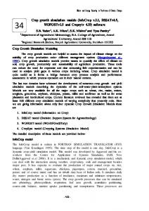
units considered as homogeneous to which the model is applied to get simulated values. Spatialisation of crop models needs to link different scales: for example, the scale on which the processes are described by the model, the scale on which input data or information (model parameters and input variables) must be available, or the scale on which output results are expected or sought. Thus, spatialisation often requires some kind of change of scale, for example from the scale of validity of the model to the support unit of the model predictions or from the support unit to the extent. Often, instead of “scale change” one talks of “upscaling” (or “downscaling”). Nevertheless, for Bierkens et al. [5], “upscaling” specifically means increasing the support, which we refer to as “aggregation” (and “downscaling” by “disaggregation”) (Fig. 1). On the other hand, expressions such as “a crop model is scaled-up from the field to the regional scale” [49] associate “upscaling” with increase in extent. Often, crop models are calibrated on the field scale and then used to estimate the evolution of some variables for this field.

Spatialising crop models

209

Figure 1. Basic operations involving extent coverage and support (from Bierkens et al., 1997).

In this instance, the field is both the extent and the support of the study. When these models are used to make decisions at a regional level (for example to map nitrate leaching), the extent of the study is no longer the field. The input data, at least in part, can no longer be determined for each field of the region. It is then often supposed that many fields have the same characteristics and therefore the same input data can be used to run the crop model for all of them. The support unit can then be considered as a set of fields, although the measurement unit of input data remains unchanged. The scale change here corresponds to the passage from a small support unit (a field) to a bigger one (a set of fields). This is aggregation or “upscaling”, and this change of support is accompanied by a change of extent (from the field to the region). On the other hand, the scale change involved in using a crop model for precision agriculture corresponds only to a change of support (one passes from a field to a homogeneous zone within the field), without any change of extent (which remains the field). Thus spatialisation of a crop model is linked to scale change analysis. Scale change corresponds to two opposite problems, the passage from a local to a global scale and vice versa. When the modelling scale changes, it may imply both a change in the scale of data observations (input data, output data or “validation” data), and a change in the structure of the modelling approach. The latter change is well known in the field of hydrodynamics, where water flow is described by the Navier-Stokes equations on the soil pore scale, and by Darcy’s equation on the scale of the soil column. Specifically regarding crop models, the equations of the crop models are established on elementary surfaces (plots of the order of one m2) or even under

controlled conditions in the laboratory. But often crop modelling is sought on the field scale. In this instance, there is a change of modelling scale. Most approaches assume that the structure of the model can remain similar and that it is possible to estimate effective values of the model parameters on the upper scale. In practice, the parameters of the model are estimated by calibrating the model with data observed on the scale of an agricultural field. In applications over a region, there is no such calibration step because the objective is not to erase the heterogeneity of the region. Similarly, in precision farming, homogeneous zones within the field are identified in order to take into account the within-field variability. The model can be applied to each of these zones. The models are then kept unchanged, and the scale change concerns mainly the input and/ or output data.

3. MAIN ASPECTS OF SPATIALISATION METHODS Assuming that the natural spatial scale of a crop model is a field plot and that the extent of the study is a collection of field plots (a drainage basin, an administrative region, etc.), spatialisation and/or spatial aggregation can be situated at three levels: (i) determining input data, (ii) accounting for the interactions between field plots, and (iii) evaluating the results. The first point deals with the problem of being able to simulate crop development for all individual fields. It requires the input data specific to each simulated field. Because crop models do not take into account specific processes concerning a larger scale

210

R. Faivre et al.

than the field, the second point involves coupling the crop model with a model that explicitly simulates the spatial determinism of some processes like, for example, those involved in a watershed hydrological functioning. Another solution is to control or update the simulated values using observations of the entire region, with satellite data, for example. Because crop models are validated at the field plot level, the third point concerns the problem of evaluation of the spatialisation process when the results concern a large area. 3.1. Determining input data throughout the extent As a simplified representation of the soil-plant-atmosphere system, a crop model refers to a locally limited environment (local scale of the homogeneous field) and in particular soil and climate conditions and crop management. In the case of the application of such a model on the scale of a heterogeneous field, a farm, a region or a country, the environment of the SPA system becomes variable, not only in time but also in space. The soil varies in depth, texture, and slope, climate, in particular rainfall, is variable and finally, management practices (soil tillage, irrigation, fertilisation, choice of cultivar, etc.) also vary. It has been shown that the validity of crop model predictions, summed or averaged over a region, depends on the quality of the representation of the spatial variability of the input data [20]. Thus moving from a homogeneous field to a larger scale or to a heterogeneous field requires incorporating additional environmental heterogeneity. Two main types of input data can be distinguished. The first includes the environment characteristics. They are essential since the basis of a crop model is to represent the interactions between biological factors and environment. A second type of data includes the technical details of management practices. 3.1.1. Environmental data The major environmental data necessary for running crop models are climatic variables (temperatures, precipitation, radiation and potential evapotranspiration) and soil properties. In general these quantities are not known everywhere and on every scale. They are measured or estimated on given spatial supports (soil profiles and meteorological stations) at a limited number of sites within the study area. For crop modelling purposes it is therefore necessary to estimate their values on the scale of every simulation unit within the simulation area. This implies some kind of spatial estimation. Various techniques and methods have been developed and applied for soil and climate data. They are very diverse and may be distinguished by the kind of model of spatial variation they are based on. Three groups of approaches may be roughly distinguished. • A first group of methods is based on models of spatial variation that can be classified as traditional and that do not consider random components. This is the case of many traditional choropleth mapping methods based on terrain inventories and surveys which define and map classes of soils, vegetation and climates, and assume that the property of interest is best estimated by the class mean at all sites within a given class. Examples of choropleth mapping are the classical soil mapping techniques, of which a review was proposed by Legros [37]. Other techniques such as

Thiessen polygons, trend analysis or arbitrarily weighted averages of data also belong to this first type of method. They have been extensively used for mapping soil and climate variables (e.g. [12, 29]). • A second group of methods assumes statistical models of spatial variation. The most well-known set of methods of this kind are the geostatistical methods. They are well described in several textbooks, such as, for example, those by Journel and Huigbregts [26], Webster and Oliver [57] and Goovaerts [18]. Their main advantages are to provide sound spatial estimates from a statistical point of view (unbiasedness and minimum variance), to take into account the spatial dependence between the data and to propose an estimate of the prediction error. The most popular of the geostatiscal methods is kriging whose predictor of a property at a given site is no more than a weighted average of the observed values at neighbouring sites. Several forms or extensions of kriging have been developed to cope with different kinds of variables: continuous and categorical, with normal, log-normal and undefined density distributions. In many applications to soil and climate variables, geostatistical methods have been shown to perform better than most other methods (e.g. [12] for rainfall mapping; [54] and [55] for soil texture mapping). They best apply to variables that exhibit stationary and continuous spatial variations. But in the case of discontinuous spatial variations, their performance was shown to be poorer (e.g. [54]). • The third group of methods relies on process-based models of spatial variation. In this case, the spatial estimation of a variable is made by simulating the processes that control the variable. For example, the simulation of soil formation on the landscape scale can provide a prediction of the actual spatial variation of soil properties (e.g. [41]). Atmospheric 3D modelling that accounts for lateral energy fluxes between fields can be used to predict the spatial variation of the local atmospheric boundary conditions of a crop model (e.g. [11]). But the development of this kind of processbased approach is still at a very early stage and cannot be considered operational yet for providing input data to crop models. In many situations, the number of available measurements of soil and climate input data is very small and insufficient to allow for accurate spatial predictions over the simulation area, whatever the performance of the mapping method used. This is so especially because of the large costs involved in measuring these data. Consequently, several approaches have been developed to investigate whether surrogate data, that are already available in existing databases or easily measurable at high spatial densities, can help in spatially predicting the variation of the required soil and climate input data to environmental models. They are of two kinds. The first one corresponds to the development of empirical or theoretical models that use the surrogate data at a site to predict the data of interest at the same site. This enables one to increase the spatial set of data for subsequent mapping. Examples of this are pedotransfer functions that use basic soil data from soil surveys, including soil morphology, soil texture, structure, organic matter content, etc., to predict more difficult-to-measure soil data such as soil water retention curves or soil hydraulic conductivity. A review of pedotransfer functions is available in McBratney et al. [38]).

Spatialising crop models

Although these functions provide only approximate results, they are often used on regional scales to parameterise crop models (e.g. [14, 30]). Another example is the assimilation of remote sensing data in a 1D model describing the transfers between soil-vegetation-atmosphere (SVAT) for estimating the local climatic data, taking into account the effect of land-use [10]. The second approach is to use the information about the spatial structure of the surrogate data to improve the spatial estimation of the variables of interest. Several techniques exist; they are most often extensions of the spatial estimation methods described above. For example, the AURELHY method [3] improves the spatial estimation of precipitation by taking into account the landscape relief through a multivariate analysis. Similarly, Monestiez et al. [43] used a special form of kriging, namely kriging with an external drift, to account for local environmental conditions of the measurement sites in the mapping of air temperature. A last example is the use of outputs of large scale numerical weather prediction (NWP) to take into account the weather types when mapping precipitation [1, 39]. The use of surrogate data, especially remote sensing data, to overcome the lack of required input data when running environmental models is very promising. A last issue when mapping soil and climate input data is the problem of change of support when the measurement support unit differs from the crop model support unit (simulation unit). Because the measurement units are generally smaller than the simulation units, the problem is the upscaling of the observed or mapped input data. This requires some knowledge about the way the variables can be averaged in space, which most often raises difficult theoretical problems. For example, how to calculate the mean temperature over a squared kilometre when land-use heterogeneities occur? It is a problem of upscaling by aggregation. But in some cases, the change of scale can also be the other way round (downscaling), particularly when the simulation area is very large. For example, to obtain predictions on the Indian sub-continental scale, Priya and Shibasaki [47] estimated the necessary local information (climate and slope on a 1-km grid) by using information available on a wider scale (meteorological stations of the national network and a digital terrain model with a large grid), using a purely statistical approach. Finally, it is important to stress that, whatever the method used, the fact of estimating model input data throughout the extent introduces errors in the model inputs, as illustrated by several examples reported by Hansen and Jones [20] and Russell and Van Gardingen [49]. One example [49] concerns climatic zoning that can be used to determine weather data at various locations of a region. Weather data from the reference meteorological station of each zone are used for sites located within the zone. If the zoning is drawn up for cereals, it may not be adapted to other crops (forage, for example): (i) because conditions after cereal harvest have not been taken into account in the classification, although they influence forage growth, and (ii) because the choice of the representative meteorological station is based on the spatial distribution of cereal crops, which may be different from that of forage because of different climatic requirements. Errors in the model inputs are likely to be propagated to outputs [32, 33].

211

3.1.2. Management data Management data include crop species, variety, sowing date and density, irrigation, fertilisation and possibly crop protection and soil tillage information. They are discontinuously distributed in space. In fact, it is the spatial distribution of management practices that determines the boundaries of the fields. The management data also vary from year to year. In a given field, different crops follow one another. Finally, management data result from decisions taken on different scales, including the farm, the cooperative, the collective organisation for irrigation, etc. At each of these levels, management decisions for the various fields are interdependent [4, 45]. This complexity is the reason that spatial representations of management data are rare. Often one simply uses values corresponding to typical or recommended practices to run the models [14, 20]. Nevertheless, it is very important to distinguish irrigated zones from non-irrigated ones, and to include the distribution of sowing dates and the range of varieties used in a region. If the spatial distribution of crops within the considered area has no effect on the simulated process, and if the analysis of the determining factors suggests it, it is possible to simply distribute the management practices in space according to a law of probability [42]. This approach was adopted by Leenhardt and Lemaire [31] for the sowing dates and by Mignolet et al. [40] for crop rotations. These two studies combine segmentation of the geographic space and sampling from probability distributions. An alternative approach to collecting information regarding agricultural practices relies on the use of remote sensing. Historically, remote sensing has widely been used to obtain landuse maps, which provide a description of the spatial distribution of crops. More recently, it has provided a means to estimate the exhaustive distribution of techniques difficult to observe because of their transient nature (e.g. sowing date and nitrogen applications) and their cost of acquisition. The principle consists of re-estimating parameters (and/or input data). An example is given for sowing and emergence dates by Guérif and Duke [19] and Launay [28], where they compare LAI values simulated by the crop model and the outputs of a reflectance model applied to the remote-sensing data. 3.2. Accounting the interactions between field plots Scale change implies the consideration of new processes and properties, emerging on the scale considered and revealed by the extension of the system considered. Such emerging processes or properties influence the SPA system but are not represented by the models developed on the local scale for homogeneous fields. These processes can concern physical transfers between neighbouring units, including: water transfer between fields, pathogen propagation, weed or GMO diffusion, etc. The interactions between fields can also result from the multiplicity of actors in a region and from the decisions they make. They arise because, on this scale, human and economic sub-systems cannot be neglected. For example, on the scale of an irrigated area, the water resource must be allocated between farmers. On the farm scale water allocation but also other management decisions are interrelated between fields due to the constraints of labour and equipment. Thus, when a model, developed on the local scale, is used on a larger scale, the results

212

R. Faivre et al.

become even more error-prone because they do not take into account the phenomena appropriate for this scale. Although the two approaches presented hereafter can provide solutions, the difficulty of spatialising crop models when strong spatial interactions exist between fields must be emphasised. When runoff or propagation of pathogens are considered, the relative locations of fields, as well as their sizes, are essential. For example, in an area where the proportion of different crops are fixed runoff will be different depending on the sizes of the fields. This will also affect biological diversity. The spatial structure gives to the system properties that cannot be directly accounted for by the crop models. To account for spatial interaction between fields, the most natural approach is to interface the crop model with a model that represents these spatial interactions. Nevertheless, such an interface is not without difficulties. First, it requires an exchange of data between the two models at each time step during the simulation process, while existing crop models are generally structured to simulate directly an entire growing season [2]. Second, on larger scales (farm, watershed or region), several crops are concerned, while crop models are generally developed for one species. Embedding crop models into models of three-dimensional hydrology, intercrop competition or farm operations would require restructuring the models so that different crops could be simulated in parallel and that information exchange could be possible at each time step of simulation between the models. Although this is possible, the difficulty of reorganising model code and the need to repeat the exercise after each model revision suggests that combined models of these higher-level systems will not be sustainable without a commitment on the part of the crop-modelling community to develop and maintain an appropriate modular structure [20]. An indirect approach to account for interactions between field plots consists of accounting for the spatial variability of the model state variables at particular moments of the crop cycle, rather than modelling explicitly spatial interactions. Injecting remote-sensing information into the model is the most common way to do this. This refers to data assimilation reviewed by Pellenq and Boulet [46]. But here, the information is used to force the crop model to be consistent with the observed data over the course of the growing season [15]. Data assimilation implies that communication between the data and the model occurs during the course of the simulation (that is, during the course of the crop cycle), which poses computer problems similar to those evoked above. However, this technique does not require a complete reorganisation of the model. 3.3. Evaluating the simulated results When a crop model is applied to a large area, the overall precision of the predictions results not only from the quality of the model itself, but also from the quality of the methods of acquisition of the input data, of the choice of the units of simulation, and of the calibration of the model. In the previous paragraphs, we underlined the importance of errors affecting input data because of the necessity of involving estimation methods over large areas. It is also important to note that these methods (pedotransfer functions, interpolation meth-

ods, remote-sensing assimilation data or sampling from distributions without any spatial constraint) can generate a spatial structuration of crop model output prediction errors. Evaluation of the overall results is possible in principle but is often problematic in practice. The most common problem is the quality of the so-called “validation” data. These data are observed data, but generally their reliability can be questioned (as is the case for the input data), which reduces the pertinence of the comparison of observed and simulated data. For example, to validate the ISOP model which estimates grass production for every forage region, Rabaud and Ruget [48] used estimations of production made a posteriori by local experts. There thus arises a problem of reliability of data (varying from one expert to another, depending on his/her own memory). Similarly, Faivre et al. [15] simulated wheat production but, for validation, they only had at their disposal statistics for the part of the production collected for commercialisation. In addition, they have a problem of discordance between spatial units: simulations are performed for 1 km2 support units (satellite pixels), while validation data are available on a communal basis. Besides, to estimate the quality of forecasts of total water demand for irrigation in a region, Leenhardt et al. [36] use data relative to farmers who subscribe to a collective irrigation system, while in the study area, there are also farmers who irrigate from their own reservoirs. There is therefore a discordance between the simulations (relative to the whole extent of the study area) and the observations (corresponding to that part of the area cultivated by farmers who irrigate from a collective system). Furthermore, within these “collective” irrigators, some receive water from collective pumping plants whose daily volume can be obtained, while others use individual pumps and only the total volume to the end of the experiment is available. Thus none of the validation data sets covers by itself the full spatial extent considered, that is, the whole irrigated region including both collective and individual irrigators, nor the full temporal extent, that is, the entire irrigation campaign with a daily time step. Actually, the term “evaluation” is more appropriate than “validation”. Rather than evaluating spatialised models by comparing predictions with imprecise observations, it is possible to evaluate them by considering if the objective is attained. In particular, does the model allow one to make decisions correctly? For example, Leenhardt et al. [36] verified, for a past year for which water management decisions failed, that a regional irrigation demand prediction model was able to predict the delay in irrigation demand that was the cause of wrong decisions. The model would then have been able to allow the water manager to anticipate the difficulties and would have helped him to make better decisions by improving the estimation of the remaining potential irrigation demand. A global evaluation gives an idea of the reliability of the results, but does not indicate how to improve them since the sources of error are not identified. To go further, it would be possible to study each individual source of error and its propagation through the model. The contribution of each type of error to the total error of the simulation result could then be identified. This type of analysis would also make it possible to choose the most adequate method of data acquisition, taking into account the effect of error in each type of data on the precision of the results. Analytical methods of decomposition and of propagation of error exist for linear models (cf. for example

Spatialising crop models

213

Figure 2. Decision-tree with four major classes of upscaling methods (from Bierkens et al., 1997).

[23]). For crop models, which are strongly nonlinear, these methods do not apply. The procedure then becomes very complex. Indeed, no complete analysis of sources of error and of their propagation has been conducted for spatial applications of crop models. Nevertheless, the procedure has been illustrated by Leenhardt and Voltz [32] for one kind of crop model input data, namely soil water properties. The aim was to choose the method of acquisition of such data, that is, what resolution for the soil map, what estimator of the water properties within the mapping units? A more complete approach but without specific application to crop models is given by Crosetto et al. [13] and by Tarantola et al. [53]. They propose an application of uncertainty and sensibility analyses to GIS-based models in order to estimate the precision needed for the various types of data. The objective is to obtain results with a precision within limits acceptable to the user, thus allowing decision-making.

4. WITH REGARD TO SCALE CHANGE Since extent and support are not on the same scales (homogeneous plot for the latter and region for the former), analysis in terms of scale change seems to be a good means of presenting the approaches of spatialisation of crop models. The decision-

tree proposed by Bierkens et al. [5] (Fig. 2) can be a good support for discussing the different studies presented in the previous section. One of the most common strategies is to look for exhaustive information all over the extent at the crop model support unit level (field) in order to simulate everywhere, and then to aggregate results to obtain information on the extent scale. This methodology corresponds to class 1 of the decision-tree. It is represented in Figure 3, way A, corresponding to a “calculate first, average later” strategy as mentioned by Bierkens et al. [5]. In Section 3.1.1, we described the methods for spatialising environmental input data, with a first view of the problem of scale change. These methods mainly correspond to a change of coverage (see Fig. 1) where the most common method is interpolation (Fig. 3, way Au). To characterise the soil typology at the necessary crop model support unit, one needs to proceed, from the original databases, to different scale change modes (Carré [9], ways Ad or Au). When technical input data are involved (see Sect. 3.1.2), interpolation methods are inadequate when local information concerning management is available. When the coverage rate of these technical information is not high enough, the use of assimilation techniques of remote-sensing data allows the modeller to estimate actual technical input data as Guérif and

214

R. Faivre et al.

Figure 3. Strategies for upscaling a crop model: upscaling outputs (way A), upscaling inputs first (way B).

Duke [19] did for the emergence dates, which corresponds to class 1 of the decision-tree (Fig. 2). In general, local information concerning management is not available. Representative management practices are used in the course of spatialising crop models. This corresponds to class 2 in the decision-tree. The meaning of “easily” in the question of Bierkens et al. [5] (“Can the model be easily applied at many locations?”) should be clarified. In the case of technical input data, it is numerically easy to apply the model but information is missing. Depending on other input data, two main strategies are used. If environmental data are also classified in different soil types, generally no spatialisation is performed [14]: all combinations of soil types and management types are simulated on the crop model scale and upscaled by weighting the results of each combination (Fig. 3 way A). If environmental input data are spatialised, i.e. if available for all the plots of the extent, the recommended management practice is used for all plots [15], i.e. scale change only concerns environmental input data while technical input data is constant over the extent. An alternative could be to spatialise management data by drawing at random from a known distribution of practices (generally available in an agricultural administrative region, see [31] and [40]); such a strategy should be used when spatial dependencies exist between plots (e.g. water flux between field plots). The strategies presented above consist of spatialising input data for all the support units of the extent, then of running the crop model for all these support units and finally of aggregating the outputs over the extent. Another strategy, implying strong hypotheses, consists of applying the model to some support units and then of extending the results to the extent by some method of interpolation (Fig. 1, Change of coverage). This is the approach implemented by Sousa and Pereira [50] to get water requirements for potatoes for a region. The outputs obtained by simulation at the locations of meteorological stations were then extended by spatial interpolation using kriging. Interpolation is based on the assumption that outputs are spatially structured (often varying continuously in space). In this application, water requirements are assumed to depend on cli-

matic factors only. However, in most applications of crop models, such an assumption is not realistic: as noted before, agricultural practices vary in space discontinuously with no known spatial structure. Therefore, there is no reason to suppose that outputs vary continuously. We presented above the spatialisation of crop model input data in order to predict outputs for all crop model support units. It could also be possible to spatialise crop model state variables. The same hypotheses of spatial structuration are necessary. More, spatialising intermediary (state) variables is very timeconsuming. Assimilation from exhaustive information over the extent is a means of overcoming these problems. It allows the updating of some of the simulated state variables in the course of the simulation. It is another method of assimilation, different from that used by Guérif and Duke [19] which estimates input data only. Scale change is often necessary due to a gap between the observed data support unit and crop model support unit. We are in the same configuration as in Figure 3, but replacing “crop model input data” with “crop model state variables”. Faivre et al. [15] are concerned with scale change to match the support unit of observed data and the crop model support unit. They first unmixed data to recover the specific value of the considered crops [16]: in the coarse satellite data of 1 km2 support unit (pixel), data consists of aggregated values of different types of crops. The scale change (way Ad in Fig. 3) is carried out when the average value of the observed data in the pixel is affected by each field (crop model support unit). Another problem relative to scale change is the spatial adequacy between evaluation data and crop model outputs over the extent. In Rabaud and Ruget [48], the validation is performed on the same support; validation data and output data are aggregated over the same extent. In Faivre et al. [15], validation data is available on an intermediary support unit (an administrative communal support unit), lower than the extent (region) but larger than the crop model support unit (field). Here, for communal and regional evaluations, a change of support by aggregation is necessary. In Leenhardt et al. [36], there is a difference of coverage: validation is based on a sample of the extent (Fig. 1, change of coverage). In terms of scale change, all work relative to spatialisation of crop models concerns only data, but never the model itself. Besides, simulations are always performed on the scale of the crop model (way A in Fig. 3), never on the scale of the target (way B in Fig. 3). Consequently, input data spatialisation methods (cf. Au et Ad in Fig. 3) and the upscaling methods of output data should benefit from the scale-change point of view. Therefore, the general principles of scale-change methods can be useful. The specificity of crop model spatialisation is that, most often, two scale changes occur: one on the input data, the other on the outputs. Input data scale change can be downscaling or upscaling. Generally, output data scale change is upscaling only (by aggregation to have global information). The common strategy consisting of simulating everywhere should be chosen either because of its better efficacy or because it respects spatial structurations that are difficult to account for differently. A way of checking the efficacy of this strategy would be to compare simulated and observed spatial variations. This would need

Spatialising crop models

information over the whole extent on the support unit scale, which is rarely the case. An alternative would be to disaggregate global information (often concerning the entire extent), taking into account some spatial dependence models. This is specifically addressed in the downscaling methods issues. 5. BY WAY OF CONCLUSION The “spatialisation of crop models” has been implemented in a number of applications. Different techniques have been used but it appears that there is a lack of analysis of the methods and strategies and of the requirements. Spatialising crop models requires a large amount of geographical information. This is why Heineman et al. [22] and Nicoullaud et al. [44], for example, coupled crop models to a geographical information system (GIS). We can see, with this analysis in terms of scale change, that this need for data can be decreased. A first solution is to use spatialisation techniques such as interpolation methods. Another one is to consider another strategy, such as the way B described in Figure 3. This new strategy would consist of calculating a mean temperature or using representative types and then simulating with these synthetic data. This is possible because a crop model has no dimension: it simulates the outputs (for example, the mean yield) per unit of area, that is, it can be used whatever the support unit of input data. In fact, the processes represented in a crop model (and assumed to be exact) are considered as being applicable only for a homogeneous support unit of the size of a field plot. A crop model is developed for a homogeneous simulation unit, generally the field plot. It takes into account only the processes that are significant on such a scale (the field). When the crop model is used on a larger extent, we have to deal with emerging processes, for example fluxes between fields. In this case, it is possible to interface the crop model with another kind of model: a hydrological model to account for lateral water flows [2], farm system model to account for constraints due to work organisation, etc. Contrary to what Bierkens et al. [5] proposed (class 4 in Fig. 2), the crop model is complexified. The corresponding question in the decision-tree should be: “shall we continue to apply the crop model as it is or shall we create a new model in which the crop model is only a sub-part?” An alternative to complexification is the use of assimilation, as noticed in Section 4. The proposition of Bierkens et al. [5], that is, simplifying the crop model, is in fact never considered. Although there exist a number of applications of crop model spatialisation, there is a crucial lack of operational and transferable tools adapted to this problem. Efforts exist but are not coordinated. In most examples, the interfaces are partial and not automated, which does not make the tool easily transferable to other researchers. These studies are often specific to one application; that is, they consider one particular model, they use one particular set of data from one study site, they address one specific question. In order to formulate a general spatialisation approach, one idea would be to combine the different points of view in terms of processes to be modelled, which implies having a multidisciplinary team working at and observing the same study site. The existence of a common study site where researchers of different disciplines would work could be a good

215

opportunity (i) to test advanced techniques, (ii) to evaluate the impact on predictions of different sources of error (corresponding to different methods of input data acquisition), and (iii) to study the techniques that should be combined to develop decision support systems. The recent creation of long-term observation experiments by research organisations in France (the Environmental Research Observatories, “ORE”, and the regional working zones, “zones atelier”) could provide the opportunity to achieve progress in crop model spatialisation. These studies would need to be viewed through the prism of the scale-change analysis. All the scientific questions evoked here are under study and in the present paper we attempt to provide a framework for analysing the spatialisation of crop models. To that extent, this paper is to be considered as a contribution to the great debate concerning the use of crop, and more generally, vegetation models on a large scale. Acknowledgements: The authors acknowledge the Department “Environnement et Agronomie” of the Institut National de la Recherche Agronomique (INRA) for having funded the seminar. We thank the authors (Bierkens M.F.P., Finke P.A. and de Willigen P.) and editor (Kluwer Academic Publishers) of the book “Upscaling and downscaling methods for environmental research” for authorising the use of some figures. We appreciated the comments and proposals of the two reviewers.

REFERENCES [1] Bardossy A., Plate E.J., Space time model for daily rainfall using atmospheric circulation patterns, Water Resour. Res. 28 (1992) 1247–1259. [2] Beaujouan V., Durand P., Ruiz L., Modelling the effect of the spatial distribution of agricultural practices on nitrogen fluxes in rural catchments, Ecol. Model. 137 (2001) 93–105. [3] Bénichou P., Le Breton O., Prise en compte de la topographie pour la cartographie des champs pluviométriques statistiques : la méthode Aurelhy. Agrométéorologie des régions de moyennes montagnes, Coll. INRA n° 39, 16–17 avril 1986, 1987, pp. 51–68. [4] Biarnès A., Rio P., Hocheux A., Analyzing the determinants of spatial distribution of weed control practices in a Languedoc vineyard catchment, Agronomie 24 (2004) 187–196. [5] Bierkens M.F.P., Finke P.A., de Willigen P., Upscaling and downscaling methods for environmental research, Kluwer Academic Publishers, Dordrecht, 2000. [6] Boote K.J., Jones J.W., Pickering N.B., Potential uses and limitations of crop models, Agron. J. 88 (1996) 704–716. [7] Brisson N., Delécolle R., Développement et modèles de simulation de culture, Agronomie 12 (1991) 253–263. [8] Brisson N., Mary B., Ripoche D., Jeuffroy M.H., Ruget F., Nicoullaud B., Gate P., Devienne-Barret F., Antonioletti R., Durr C., Richard G., Beaudoin N., Recous S., Tayot X., Plenet D., Cellier P., Machet J.M., Meynard J.-M., Delécolle R., STICS: a generic model for the simulation of crops and their water and nitrogen balances. I. Theory and parametrization applied to wheat and corn, Agronomie 18 (1998) 311–346. [9] Carré F., Cartogénèse des sols et changements d’échelle – Application dans la région de La Rochelle sur une base de données pédologiques de plusieurs milliers d’observations (Quantitative soil mapping and scaling – Application to a French soil database (La Rochelle area) with thousands observations), Ph.D. thesis of the Institut National Agronomique Paris-Grignon, 2003. [10] Courault D., Clastre P., Cauchy P., Delécolle R., Analysis of spatial variability of air temperature at regional scale using remote sensing data and a SVAT model, in: 1st Int. Conf. of Geospatial

216

R. Faivre et al.

Information in Agriculture and Forestry, Decision support, technology and applications, Lake Buena Vista (USA), 1–3 June 1998, Vol. 2, pp. 149–156.

[31] Leenhardt D., Lemaire P., Estimating the spatial and temporal variability of sowing dates for regional water management, Agric. Water Manage. 55 (2002) 37–52.

[11] Courault D., Lacarrère P., Clastre P., Lecharpentier P., Jacob F., Marloie O., Prévot L., Olioso A., Estimation of surface fluxes in a small agricultural area using the 3D atmospheric model Meso-NH and remote sensing data, Can. J. Remote Sens. 29 (2003) 741–754.

[32] Leenhardt D., Voltz M., Évaluation de l’erreur induite par l’utilisation de cartes de sol pour la spatialisation d’un modèle de culture, in: Leenhardt D., Faivre R., Benoît M. (Eds.), Actes du séminaire “Spatialisation des modèles de culture”, Toulouse, 14–15 janvier 2002.

[12] Creutin J.D., Obled C., Objective Analyses and Mapping Techniques for Rainfall Fields: An Objective Comparison, Water Resour. Res. 18 (1982) 413–431. [13] Crosetto M., Tarantola S., Saltelli A., Sensitivity and uncertainty analysis in spatial modelling based on GIS, Agric. Écosyst. Environ. 81 (2000) 71–79. [14] Donet I., Le Bas C., Ruget F., Rabaud V., Guide d’utilisation d’ISOP, Agreste Chiffres et Données Agriculture, n° 134, 2001, 55 p. [15] Faivre R., Bastié C., Husson A., Integration of VEGETATION and HRVIR into yield estimation approach, in: Gilbert Saint (Ed.), Proceedings of “Vegetation 2000, 2 years of operation to prepare the future”, Space Application Institute and Joint Research Center, Ispra, Lake Maggiore (Italy), 3–6 April 2000, pp. 235–240. [16] Faivre R., Fischer A., Predicting crop reflectances using satellite data observing mixed pixels, J. Agric. Biol. Environ. Stat. 2 (1997) 87–107. [17] Gomez E., Ledoux E., Démarche de modélisation de la dynamique de l’azote dans les sols et de son transfert vers les aquifères et les eaux de surface, C.R. Acad. Agric. France 87 (2001) 111–120. [18] Goovaerts P., Geostatistics for natural resources evaluation, Oxford University Press, Oxford, 1997. [19] Guérif M., Duke C., Calibration of the SUCROS emergence and early growth module for sugarbeet using optical remote sensing data assimilation, Eur. J. Agron. 9 (2000) 127–136. [20] Hansen J.W., Jones J.W., Scaling-up crop models for climate variability application, Agric. Syst. 65 (2000) 43–72. [21] Hartkamp A.D., White J.W., Hoogenboom G., Interfacing Geographic Information Systems with Agronomic Modeling: A Review, Agron. J. 91 (1999) 761–772. [22] Heinemann A.B., Hoogenboom G., Faria de R.T., Determination of spatial water requirements at county and regional levels using crop models and GIS. An example for the State of Parana, Brazil, Agric. Water Manage. 52 (2002) 177–196. [23] Heuvelink G.B.M., Burrough P.A., Stein A., Propagation of errors in spatial modelling with GIS, Int. J. Geogr. Inf. Syst. 3 (1989) 303–322. [24] Hoogenboom G., Contribution of agrometeorology to the simulation of crop production and its applications, Agric. For. Meteorol. 103 (2000) 137–157. [25] Jones C.A., Kiniry J., CERES-MAIZE, a simulation model of maize growth and development, Texas A and M University Press, 1986. [26] Journel A.G., Huijbregts C.J., Mining Geostatistics, Academic Press, New York, 1978. [27] Lal H., Hoogenboom G., Calixte J.P., Jones J.W., Beinroth F.H., Using crop simulation models and GIS for regional productivity analysis, Trans. ASAE 36 (1993) 175–184. [28] Launay M., Diagnostic et prévision de l’état des cultures à l’échelle régionale : couplage entre modèle de croissance et télédétection. Application à la betterave sucrière en Picardie, Ph.D. thesis, Institut National Agronomique Paris Grignon, 2002. [29] Laslett G.M., McBratney A.B., Pahl P.J., Hutchinson F., Comparison of several spatial prediction methods for soil pH, J. Soil Sci. 38 (1987) 325–341. [30] Leenhardt D., Errors in the estimation of soil water properties and their propagation through a hydrological model, Soil Use Manage. 11 (1995) 15–21.

[33] Leenhardt D., Voltz M., Bornand M., Propagation of the error of spatial prediction of soil properties in simulating crop evapotranspiration, Eur. J. Soil Sci. 45 (1994) 303–310. [34] Leenhardt D., Voltz M., Rambal S., A survey of several agroclimatic soil water balance models with reference to their spatial application, Eur. J. Agron. 4 (1995) 1–14. [35] Leenhardt D., Trouvat J.-L., Gonzalès G., Pérarnaud V., Prats S., Estimating irrigation demand for water management on a regional scale. I. ADEAUMIS, a simulation platform based on bio-decisional modelling and spatial information, Agric. Water Manage. (in press). [36] Leenhardt D., Trouvat J.-L., Gonzalès G., Pérarnaud V., Prats S., Estimating irrigation demand for water management on a regional scale. II. Validation of ADEAUMIS, Agric. Water Manage. (in press). [37] Legros J.-P., Cartographie des sols. De l’analyse spatiale à la gestion des territoires, Coll. Gérer l’environnement, Presses polytechniques et universitaires romandes, 1996. [38] McBratney A.B., Minasny B., Cattle S.R., Vervoort R.W., From pedotransfer functions to soil inference systems, Geoderma 107 (2002) 55–70. [39] Merlier C., Mean daily precipitation values over France related to 700 mb geopotential heights patterns, in: Data spatial distribution in meteorology and climatology, COST Action 79, WMO, EUR 18472 EN, Volterra, 1997, pp. 65–71. [40] Mignolet C., Schott C., Benoît M., Spatial dynamics of agricultural practices on a basin territory: a retrospective study to simulate nitrate flow. The case of the Seine basin, Agronomie 24 (2003) 219–236. [41] Minasny B., McBratney A.B., A rudimentary mechanistic model for soil formation and development. II. A two-dimensional model incorporating chemical weathering, Geoderma 103 (2001) 161– 179. [42] Moen T.N., Kaiser H.M., Riha S.J., Regional yield estimation using a crop simulation model: concepts, methods and validation, Agric. Syst. 46 (1994) 79–92. [43] Monestiez P., Courault D., Allard D., Ruget F., Spatial interpolation of air temperature using environmental context: application to a crop model, Environ. Ecol. Stat. 8 (2001) 297–309. [44] Nicoullaud B., Couturier A., Beaudouin N., Mary B., Coutadeur C., King D., Modélisation spatiale à l’échelle parcellaire des effets de la variabilité des sols et des pratiques culturales sur la pollution nitrique agricole, in: Monestiez P. (Ed.), Comptes rendus de l’AIP ECOSPACE, 1999, 13 p. [45] Papy F., Pour une théorie du ménage des champs : l’agronomie des territoires, C.R. Acad. Agric. France 87 (2001) 139–149. [46] Pellenq J., Boulet G., A methodology to test the pertinence of remote-sensing data assimilation into vegetation models for water and energy exchange at the land surface, Agronomie 24 (2003) 197–204. [47] Priya S., Shibasaki R., National spatial crop yield simulation using GIS-based crop production model, Ecol. Modell. 135 (2001) 113– 129. [48] Rabaud V., Ruget F., Validation de variations interannuelles d’estimations de productions fourragères appliquées à de petites régions françaises, in: Leenhardt D., Faivre R., Benoît M. (Eds.), Actes du séminaire “Spatialisation des modèles de culture”, Toulouse, 14–15 janvier 2002.

Spatialising crop models

[49] Russel G., Van Gardingen P.R., Problems with using models to predict regional crop production, in: Van Gardingen P.R., Foody G.M., Curran P.J. (Eds.), Scaling-up from cell to landscape, Cambridge University Press, 1997, pp. 273–294. [50] Sousa V., Santos Pereira L., Regional analysis of irrigation water requirements using kriging. Application to potato crop (Solanum tuberosum L.) at Tras-os-Montes, Agric. Water Manage. 40 (1999) 221–233.

[54]

[55]

[51] Spitters C.J.T., Van Keulen H., Van Kraalingen D.W.G., A simple and universal crop growth simulator: SUCROS87, in: Rabbinge R., Ward S.A., Van Laar H.H. (Eds.), Simulation and system management in crop protection, Simulation Monographs, Pudoc, Wageningen (Netherlands), 1989, pp. 147–181.

[56]

[52] Stöckle C.O., Martin S.A., Campell G.S., CROPSYST, a cropping systems simulation model: water/nitrogen budgets and crop yield, Agric. Syst. 46 (1994) 335–359.

[57]

[53] Tarantola S., Giglioli N., Saltelli A., Jesinghaus J., Global sensitivity analysis for the quality assessment of GIS-based models, in:

[58]

217

Heuvelink G.B.M., Lemmens M.J.P.M. (Eds.), Accuracy 2000, Proceedings of the 4th International Symposium on Spatial Accuracy Assessment in Natural Resources and Environmental Sciences. Amsterdam, July 2000, pp. 637–641. Voltz M., Webster R., A comparison of kriging, cubic splines and classification for predicting soil properties from sample information, J. Soil Sci. 41 (1990) 473–490. Van Meirvenne M., Scheldemann K., Baert G., Hofman G., Quantification of soil textural fractions of Bas-Zaïre using soil map polygons and/or point observations, Geoderma 62 (1994) 69–82. Wallach D., Goffinet B., Bergez J.-E., Debaeke P., Leenhardt D., Aubertot J.-N., Parameter estimation for crop models: a new approach and application to a corn model, Agron. J. 93 (2001) 757–766. Webster R., Oliver M., Statistical methods in soil and land resource survey, Oxford University Press, 1990. Williams J.R., Jones C.A., Kiniry J.R., Spanel D.A., The EPIC crop growth model, Trans. ASAE 32 (1989) 497–511.

To access this journal online: www.edpsciences.org