Spatio-Temporal Aggregation Using Sketches - CiteSeerX

ICDE 2004 Submission ID: 414

Spatio-Temporal Aggregation Using Sketches Yufei Tao§, George Kollios*, Jeffrey Considine*, Feifei Li*, and Dimitris Papadias† §

Department of Computer Science Carnegie Mellon University Pittsburgh, PA, USA [email protected]

*

Department of Computer Science Boston University Boston, MA, USA {gkollios, jconsidi, lifeifei}@cs.bu.edu

†

Department of Computer Science Hong Kong University of Science and Technology Clear Water Bay, Hong Kong [email protected]

time is in the past or the present), a spatio-temporal aggregate query retrieves summarized information about objects that appeared in qr during qt. We consider two cases of such queries: (i) the spatio-temporal count that returns the total number of qualifying objects, and, (ii) the spatio-temporal sum which, assuming that each object is associated with a measure, outputs the sum of the measures of the qualifying objects. For instance, a measure of interest for the mobile computing scenario is the number of phone calls, in which case the corresponding spatio-temporal sum query will return the total number of phone calls made by all users in region qr during interval qt. Obviously, the spatio-temporal count is a special case of the spatio-temporal sum, where the measure of each point is 1. The only directly-related, previous work [PTKZ02] proposes several multi-tree structures based on R-trees and B-trees (for details see Section 2.2). The shortcoming of that approach (which is also the motivation of this paper), is the so-called distinct counting problem, i.e., if an object remains in the query region for several timestamps during the query interval, it will be counted (or summed) multiple times in the result. Since the structures of [PTKZ02] store only summarized data (and, therefore, information about individual objects is lost), the problem cannot be solved by duplicate elimination techniques, but necessitates the development of alternative methods. An effective solution to the distinct counting problem is crucial for several applications because it can support a much more extensive range of decision-making queries. A natural question in traffic analysis, for example, is to ask how many cars are present in a district. The techniques of [PTKZ02] can be used to find the average number of cars during a time interval. However, the average is not adequate in analyzing the traffic volume. For example, one might find a parking garage and a busy highway with the same average number of cars, and then assert that they have similar traffic characteristics. By incorporating distinct counting, on the other hand, we can distinguish between the two cases. First, the highway will have a much higher turnover rate of cars entering and leaving, which will be directly reflected in a higher distinct number of cars. Second, this turnover rate can be quantified by comparing this number against the average. That is, if the number of distinct cars increases by x, while

Abstract Several spatio-temporal applications require the retrieval of summarized information about moving objects that lie in a query region during a query interval (e.g., the number of mobile users covered by a cell, traffic volume in a district, etc.). Existing solutions have the distinct counting problem: if an object remains in the query region for several timestamps during the query interval, it will be counted multiple times in the result. The paper describes methods that solve this problem by integrating spatiotemporal indexes with sketches, traditionally used for approximate query processing. The proposed techniques can also be applied to reduce the space requirements of conventional spatio-temporal data and to mine spatiotemporal association rules.

1. Introduction Despite the vast spatio-temporal literature that aims at retrieving objects satisfying various query predicates, most related applications are interested in aggregate information about the qualifying objects. Some examples include traffic supervision systems (i.e., monitoring the number of vehicles in a district, as opposed to their ids) and mobile computing applications (i.e., where the goal is to allocate bandwidth depending on the usage of each cell, without reference to the individual users). Although summarized results can be obtained using conventional operations on individual objects (i.e., by accessing every single record qualifying the query), as suggested in [PTKZ02], there are several reasons for the development of specialized spatio-temporal aggregation methods: (i) in some cases personal data should not be stored due to legal issues. For instance, keeping historical locations of mobile phone users may violate their privacy; (ii) individual data may be irrelevant or unavailable, as in the traffic supervision system mentioned above; (iii) although individual data may be highly volatile and involve extreme space requirements, the aggregate information usually remains fairly constant for long periods, thus requiring considerably less space for storage. For example, although the distinct cars in a city area usually change rapidly, their number at each timestamp may not vary significantly, since the number of objects entering the area is similar to that exiting. Given a rectangle qr and an interval qt (whose ending

1

position of this bit be k; then FM estimates the number n of distinct objects as n=1.29×2k, which, as proven in [FM85], is indeed an unbiased estimate, i.e., E[n]=1.29×2E[k] (where E[.] denotes the expected value of a random variable). Nevertheless, the value k thus obtained has high variance, which may lead to substantial error in the estimate 1.29×2k (note that, the estimate will double even if k varies by only 1). In order to remedy this, Flajolet and Martin propose using multiple m sketches, i.e., in this case FM requires m independent hash functions, each operating on a different sketch in the same way as described earlier. Let k1, k2, …, km denote the positions of the first 0 in the m sketches respectively; FM estimates k the distinct number n (of objects) as 1.29×∑m i=12 a, where m ka=(1/m)∑i=1(ki). As shown in [FM85], this is also an unbiased estimate, with (much better) standard error O(m−1/2), namely, smaller error is expected by using larger number of sketches. The above approach has two problems. First, the processing cost of each object is increased from O(1) (if only a single sketch is used) to O(m). Second, the requirement of multiple independent hash functions results in considerable implementation difficulty (especially for large m). Flajolet and Martin [FM85] solve both problems by proposing the Probabilistic Counting with Stochastic Averaging (PCSA) algorithm, whose pseudo-code is illustrated in Figure 2.1. The key idea of PCSA is that, for each object, we apply hash function on only one sketch that is randomly selected from the m sketches (i.e., thus the processing cost is still O(1)). As a result, each sketch is responsible for approximately n/m (distinct) objects, and this is reflected in the modified estimation formula. Specifically, given the same k semantics of k1, k2,…, km, PCSA returns 1.29m·∑m i=12 a, m where ka=(1/m)∑i=1(ki) (see [FM85] for the theoretical justification).

the average stays constant, x cars must have entered and x must have left within the time period in question. One difficulty arising from the use of direct distinct counting is that, there is no way to exactly summarize distinct objects substantially better than by simply enumerating all of them. As this is impractical in most settings, we are forced to consider approximate methods. Fortunately, there are several known approximation techniques based on compact sketches. In this paper we combine one such technique (reviewed in the next section), proposed by Flajolet and Martin in [FM85] (referred to as FM in the sequel), with spatio-temporal aggregate indexes. Although our main goal is to solve the distinct counting problem, we show that the proposed techniques can also be used for alternative tasks, such as reducing the space requirements of conventional spatiotemporal databases and mining spatio-temporal association rules. The rest of the paper is organized as follows. Section 2 surveys the previous work that is related to ours. Section 3 formally defines the problem, and describes the proposed methods. Section 4 discusses several related problems that can be solved using our technique, while Section 5 contains an extensive experimental evaluation. Finally, Section 6 concludes the paper with directions for future work.

2. Related Work We first review the FM algorithm for approximate counting as it constitutes part of our solution. Then, assuming basic knowledge of R-trees [G84, BKSS90], we describe the existing approaches for aggregate processing in multi-dimensional spaces, focusing on spatio-temporal applications.

•

The FM algorithm and counting sketch

Estimating the number of distinct objects in a dataset has received considerable attention (see [GGR03, PGF02] and the references therein). Many methods in the literature are based on the FM algorithm developed by Flajolet and Martin [FM85]. Specifically, FM requires a hash function h which takes as input an object id o, and outputs a random integer h(o) in [1,r], where r is a sufficiently large number. The probability Prob[h(o)=v] that h(o) takes a specific value v∈[0,r] depends on v (i.e., the distribution of h(o) is not uniform). Specifically, Prob[h(o)=v]=2−v, namely, for half (in expectation) of the objects, h(o)=1, and, for ¼ of them, h(o)=2, etc. Based on this idea, Flajolet and Martin propose maintaining a sketch consisting of r bits that are set to 0 initially. For each object o in the dataset, FM sets the h(o)-th bit (of the sketch) to 1. Then, after processing all objects, FM examines the resulting sketch, and finds the first bit that is still 0 (i.e., it has not been set by any object). Let the

algorithm FM_PCSA (DS, h, m, r) /* DS is a dataset; h is a random function such that, given an object o∈DS, Prob[h(o) = v ]=2−v; m is the number of sketches used; r is the number of bits in each sketch */ 1. init m sketches s1, s2, …, sm, each with r bits, all set 0 2. for each object o in DS 3. randomly pick a sketch si (1≤i≤m) 4. si[h(o)] = 1 5. k=0 6. for i=1 to m 7. for j=1 to r 8. if si[j] = 0 then k = k + j; next i; 9. return (1.29m·2 k/m ) end FM_PCSA

Figure 2.1: FM Algorithm As shown in [FM95], a proper value for r (i.e., the number of bits in a sketch) is O(log2n) (r=24 suffices for

2

most practical applications), where n is the number of distinct objects. As a result, the space consumption of the FM algorithm is O(m·log2n) when m sketches are used.

•

number is 265 in interval [4,5]. The B-tree of a non-leaf R-tree entry (e.g., R1) summarizes the aggregated data about regions in its sub-tree. For example, the first leaf entry of the B-tree for R1 denotes that the number of objects in r1, r2 (which are in the child node of R1) at timestamp 1 is 225. Similarly the first entry of the top node denotes that this number during the interval [1,3] is 685. The aRB-tree facilitates aggregate processing by eliminating the need to visit nodes totally enclosed by the query. As an example, consider the query in Figure 2.2a (with interval qt=[1,3]). Search starts from the root of the R-tree. Entry R1 is totally contained inside the query window and the corresponding B-tree is retrieved. Since the entries of the root node in this B-tree contain the aggregate data of intervals [1,3], [4,5], the next level of the B-tree does not need to be accessed and the contribution of R5 to the query result is 685. The second root entry of the R-tree, R6, partially overlaps the query rectangle qr; hence the algorithm visit its child node, where only entry R3, intersects qs, and thus its B-tree is retrieved. The first root entry suggests that the contribution of r4 for interval [1,2] is 259. In order to complete the result we will have to descend the second entry and retrieve the aggregate value of r4 for timestamp 3 (i.e., 125). The final result (i.e., total number of objects in these regions in the interval [1,3]) is the sum 685+259+125 (as mentioned earlier, the sum of aggregate data in the shaded cells of Figure 2.2b). The aRB-tree, however, does not consider duplicate elimination in the aggregate result. For example, the same set of objects may locate in r1 at timestamps 1, 2, 3, and will be counted multiple times in the query of Figure 2.2b. Therefore, it is not applicable in applications that require “distinct counting”, as is the focus of this paper.

The aRB-tree

Papadias, et al. [PTKZ02] propose the aRB-tree that is the first access method for efficient spatio-temporal aggregation. Given a set of regions r1, r2, …, rn (Figure 2.2a shows an example with n=4), they consider that the database contains the information described in Figure 2.2, where the horizontal/vertical dimension corresponds to time/regions, and the value of each cell (t,ri) denotes the number of objects in ri at time t. Consider, for example, the spatio-temporal sum query q whose rectangle qr intersects r1, r2, r4 (as shown in Figure 2.2a), and whose interval qt=[1,3]. The result equals the sum of the values in the shaded cells of Figure 2.2b. regions R1 r1

r2

r3

r4

r4

132 127 125 127 127

r

12

r

R2

qr

3

12

75

2

80

12

12

85

12

90

90

r 1 150 150 145 135 130 1

2

3

5

4

time

(a) Region extents (b) 2D view of the aggregates Figure 2.2: Regions and their aggregate data B-tree for R 2

B-tree for R 1 1 685 4 445

1 283 3 405

R-tree for the 4 225 5 220 spatial dimensions

1 225 2 230 B-tree for r1

R

1

1 445 4 265

1 150 3 145

r

1

r2

1 144 2 139

R2

3 137 4 139

B-tree for r

r

3

r4

4

1 259 3 379

4 135 5 130 B-tree for r

1 132 2 127

2

3 125 4 127

•

1 155 3 265 B-tree for r 3 1 75

2 80

3 85

4

90

Other techniques for aggregate processing

Most work in the literature considers the following problem: given a set of objects (points, rectangles, etc.) and a rectangular query window q, return the number of objects intersecting q. Efficient structures for point data include the aP-tree [TPZ02], and the CRB-tree [GAA03], which achieves the optimal performance (i.e., logarithmic query time and linear space) in the 2D space. For 2D interval objects, the MVSB-tree [ZMT+01] solves the problem in logarithmic query time, while in [ZTG02] Zhang, et al. develop a set of structures for general rectangle data with good worst-case bounds. Further, several authors [PKZT02, LM01] suggest augmenting a conventional R-tree with summary data in the non-leaf entries (in a way similar to aRB-trees) to accelerate aggregate queries for data with arbitrary extents and dimensionality. As with the aRB-tree, however, these approaches do not support distinct counting, and hence cannot be applied in our problem.

1 12

Figure 2.3: The aRB-tree In the aRB-tree, the extents of all regions (in this case r1,r2,…,r4) are stored in an R-tree. Each (leaf/non-leaf) entry of the R-tree is associated with a pointer to a B-tree that stores historical aggregate data about the entry. Figure 2.3 illustrates the aRB-tree for the example of Figure 2.2 (the minimum bounding rectangles, or MBR for short, of the non-leaf R-tree entries R1, R2 are shown in Figure 2.2a). The B-tree of r1, for example, contains 4 leaf entries (in the format (with time being the index key), corresponding to its 4 aggregate changes in history (i.e., no change at time 2). Each non-leaf B-tree entry also has the same format. The first root entry (in the B-tree for r1), for example, indicates that the total number of objects in r1 during interval [1,3] is 445, while the second entry shows that the

3

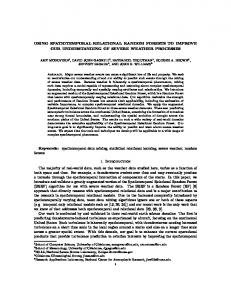
DC/DS queries precisely, requires Ω(n·T) space (n is the number of distinct objects), which is prohibitive in practice (where both n and T are massive). Our goal is to develop a structure that answers DC/DS queries approximately, consuming Ο(m·R·T·logn) space, where R is the number of regions, and m is an adjustable constant that, as explained shortly, offers tradeoffs between space, query time, and approximation accuracy. Motivated by the FM algorithm (introduced in Section 2), we maintain a sketch si(t) for each region ri (1≤i≤m) and timestamp t, that captures the (ids of) objects whose locations are in ri at t (for simplicity, we first illustrate our technique for DC queries before extending to DS processing in Section 3.3). Figure 3.1 presents the architecture of our system for distinct aggregation. At each timestamp, each object reports its id (or measure, for DS queries) to the region that covers its location. Each region has a sketch producer that is responsible for creating the corresponding sketches based on the object information, and transmits them to the database. To obtain sketches for DC queries, the producer simply performs the PCSA algorithm described in Section 2.1, while the algorithm for DS is more complex and will be discussed in Section 3.3.

Finally, approximate query answering has been addressed using various techniques such as histograms [TGIK02], sampling [CDD+01], randomized data access [HHW97], function-fitting [CR94], etc. All these methods, however, assume a single “snapshot” of the database, and do not support spatio-temporal temporal (historical) data (the only histograms with a temporal aspect focus on spatiotemporal prediction [TSP03]).

3. Distinct Spatio-Temporal Aggregation In Section 3.1, we formally define the problem, and overview the proposed methods. Then, Section 3.2 proposes the sketch index that facilitates count queries, while Section 3.3 extends the solution to sum processing.

3.1 Problem definition and solution overview We consider a set of R 2D static regions r1, r2, …, rR (the extents of two regions may overlap) as the finest aggregation granularity (e.g., cells in a mobile communication, road segments, etc.), and a set of n moving objects with distinct ids o1, o2, …, on (n>>R). Let o(t) represent the location of object o at time t. Assume that o(t) cannot be measured accurately, but instead we know the set of objects that fall in each region every timestamp, which is indeed the case in many practical applications. For example, although it is unrealistic to track the exact location of every mobile user at each timestamp, it is possible to decide which antenna cell the user is being serviced. Given an aggregate query q that specifies (i) a rectangle qr, and (ii) a time interval qt, we define the set M(q) of matching objects as: M(q) = {oi | ∃region rj & time t∈qt s.t., oi(t)∈rj and rj intersects qr} Note that, M(q) is defined through the spatial regions (i.e., the finest aggregation granularity). In particular, an object is still matching (even though it may not appear in qr during qt), as long as it appears in some region r (during qt) that intersect qr. Now we are ready to define the query types considered in this paper. Problem 3.1: A distinct (spatio-temporal) count (DC, for short) query q specifies a rectangle qr, time interval qt, and returns the number of matching objects, or more formally: DC(q) = |M(q)|. If we assume each object oi carries a measure wi (invariant with time), then a distinct sum (DS) query q specifies the same information, but retrieves the sum of the measures of all matching objects: DS(q)=∑{wi | oi∈M(q)}. ■ It is well known that, computing DC(q) exactly requires at least linear space (since the DC query is a special case of DS with measure wi=1, the same space lower bound also applies to DS). This implies that if the total number of timestamps in history is T, any solution that solves

r

sketch producers r

1

2

object ids or weights

object ids

object ids

or weights

or weights

r

3

sketches approx. results

database

aggregate queries

Figure 3.1: System architecture The sketches received by the database can be stored in a two dimensional array shown in Figure 3.3 (assuming R=4 regions). This is similar to the storage scheme in Figure 2.2b, except that each cell now contains sketches, instead of the number of objects in each region at a timestamp. Lemma 3.1: Using the sketch si(t) in cell (ri, t), we can estimate the distinct number ni(t) of objects in ri at timestamp t. ■ This lemma results from the straightforward application of the FM estimation algorithm. Namely, by identifying the position k of the left most 0 in si(t), we can estimate ni(t) as 1.27×2k. The following lemma illustrates another important property, which constitutes the rationale underlying the proposed method. Lemma 3.2: Using the OR of the sketches of c cells (rx1, t1), (rx2, t2), …, (rxc, tc), (two cells may have the same region or timestamp), we can estimate the number of

4

distinct objects o that appear in some region rxj at time tj.■ The correctness of this lemma is due to the fact that, the sketch (from the FM algorithm) for the union of several datasets, is identical to the OR of the sketch of each individual dataset. In other words, let DS be the set of objects that satisfy the condition stated in Lemma 3.2; then the sketch of DS is exactly the same as the ORci=1 sxi(ti).

leaf R-tree entry Ri, its sketch at any time t, is the OR of sketches of all the regions in the subtree (of Ri) at t. The sketch index is a dynamic structure, and its incremental maintenance algorithms are similar to those of the aRBtree (due to the similarity in their structures). R-tree for the spatial dimensions R R2 1

r B-tree for R

r 4 10000 11000 10000 10100 10100

1 11100 4 11101

r 3 01000 10000 10000 10000 11111 regions

1

1 10100 2 11100

1

r

N2 4 11100 5 10101

1 11100 4 11101

1 10000 01100 0110011100 10100 1

2

3

4

5

1 10000 2 01100

4 11100 5 10100

B-tree for r 2

time

r

3

r4 B-tree for R

N1

B-tree for r 1

r 2 10100 1000010000 11000 10001

r2

1 11100 4 11101

2

1 11000 5 11111 1 11000 3 10000

4 10100 5 11111

B-tree for r

3

1 11000 5 11111 1 01000 2 10000

5 11111

B-tree for r

4

N3

1 11000 3 10100

Figure 3.2: Conceptual sketch storage model

N4 1 10100 3 10000

Lemma 3.2 indicates a simple algorithm for approximate DC processing. Consider, for example, a DC query with rectangle qr intersecting r1, r2, r4 and qt=[1,4]. The goal is to compute the OR of the sketches in the shaded cells. In this case, the result is 11100, and since the left-most 0 is at position 4, the (approximate) result equals 1.29×24=10.32. This algorithm, however, is “conceptual”, meaning that it does not consider the actual access paths to fetch the necessary sketches, which as explained in [PTKZ02], cannot be efficiently solved using conventional data warehouses techniques due to the following reasons: (i) there is no natural ordering on the region axis, (ii) (because of the previous reason) regions intersecting qr may not be consecutive, and (iii) there is pre-defined hierarchy on regions (rendering traditional group-by techniques inapplicable). Motivated by this, in the next section we introduce the sketch index to accelerate the sketch retrieval.

4 11000 5 10001

1 10000 2 11000

3 10000 4 10100

Figure 3.3: A sketch index example

•

Query algorithm for sketch index

A straightforward algorithm for answering DC queries using the sketch index is to perform the search in a way similar to that in the aRB-tree. To illustrate this, we assume, for simplicity, the same extents of regions (r1, r2,…, r4) and non-leaf R-tree entries (R1, R2) as those in Figure 2.2a. Consider again the query q solved earlier using the “conceptual” algorithm in Section 3.1, whose query rectangle qr is as in Figure 2.2a, and interval qt=[1,4]. The search algorithm initiates a result sketch RS with all bits set to 0, and gradually updates it till the end of execution, at which point the final RS is used to perform estimation. Specifically, the search starts from the root of the R-tree. Since R1 is contained in qr, we fetch the root N1 of its B-tree, where the first entry indicates that the OR of all sketches in its subtree during [1,3] is 11100, which becomes the new value of RS. The child node N2 of the second root entry must be searched, inside which entry qualifies qt, and its sketch is OR-ed with RS (which, however, incurs no change to RS). Next the algorithm backtracks to the Rtree, and since R2 partially intersects qr, we access its child node, inside which the only entry intersecting qr is r4. Hence we search its B-tree in the same way (i.e., accessing N3 and N4) as we did for that of R5, after which the algorithm terminates with the final sketch RS=11100 (the accessed B-tree nodes are grey in Figure 3.3). The above algorithm deploys only spatial and temporal conditions (using qr and qt respectively) to prune the search space, while completely ignoring the pruning power of the sketches themselves. Notice that, in the previous example, RS is already set to 11100 (i.e., the final result) at the very early stage of the search process

3.2 Sketch Index The sketch index is similar to the aRB-tree in structure, but differs significantly in the query algorithms. Figure 3.3 shows an example (for the data in Figure 3.2), which includes an R-tree that indexes the regions (i.e., r1, r2,…, r4). Each leaf (or non-leaf) R-tree entry is associated with a B-tree that records the historical sketches of the corresponding region (or regions in its sub-tree). For example, the B-tree of region r1 consists of 4 entries (in the format ), indicating its 4 sketch changes in history (i.e., no change at time 3). The sketch 11100 of the first root entry in this B-tree equals, the OR of all the sketches (i.e., 10000, 01100) in its subtree (this rule applies to all non-leaf B-tree entries). Consider the first leaf entry in the B-tree of R1. Its sketch 10100 equals the OR for sketches of r1 and r2 (i.e., 10000, 10100, respectively) at time 1. In general, for each non-

5

(i.e., after accessing the root of the B-tree of R1). In other words, sketches of the entries subsequently visited do not affect the final result at all. Motivated by this, we observe the following pruning heuristic. Heuristic 3.1: Let RS be the current result sketch, and e a non-leaf B-tree entry whose associated sketch is se. Then, the sub-tree of e can be pruned if (se OR RS) = RS. ■ According to this rule, access to node N4 can be avoided in answering the above query, because the sketch (10100) of its parent entry satisfies 10100 OR RS (i.e., 11100) = RS. This reminds us that, in order to maximize the effectiveness of Heuristic 3.1, we should first try to set as many bits (to 1) in RS as possible, before attempting to descend any non-leaf (B-tree) entries. In general, we should “postpone” visiting any node since it may be pruned later as more bits of RS are set. Which node accesses, however, are unavoidable, and which are not? To answer this question, let SRE be the set of R-tree entries whose B-trees must be accessed. Equivalently, each entry e in SRE satisfies the following conditions: (i) its MBR is covered by query rectangle qr (or its MBR intersects qr if e is a leaf) and (ii) none of its ancestor entries satisfies (i). In the example of Figure 3.4, SRE={R1,r4}. Evidently, accesses to the roots of their respective B-trees are unavoidable. Hence we can “safely” visit all of them (in Figure 3.4, nodes N1 and N3), and examine the entries therein. Some of these entries allow us to set (possibly many) bits of RS without any further node access. The first entry of N1, for example, is one such entry, because it represents time interval (called its lifespan in the sequel) [1,3] (3 is derived from the timestamp of the next entry 4), which is contained in the query interval qt. So we can immediately update RS to its sketch 11100 (which is the OR of all the sketches in its sub-tree). Similarly, the lifespan [1,2] of the first entry in N3 is also contained in qt; hence its sketch 11000 can be used to update RS (after which RS remains 11100). Now let us consider the second entries in N1 and N3, namely, and . We are not able to decide if their sub-trees should be visited from their lifespans. As mentioned earlier, however, we can assert by Heuristic 3.1 that can be pruned, while this heuristic does not eliminate since its sketch 11101 OR RS = 11101 ≠ RS. Thus it becomes the only entry, the access to whose sub-tree seems to be “unavoidable” so far. Recall that, strictly speaking our objective (for calculating the approximate result) is not to retrieve the complete final RS. Instead, all we are interested in is merely the position of the left-most bit that is still 0. What is the possible left-most position (of the final RS) in this case (given our current RS=11100 and entry )? Clearly, the answer is 4 (i.e., the left-most 0 must be at the 4-th bit), since the first 3 bits of both RS and the entry’s

sketch are all 1. Therefore, we assert that access to the child node of this entry can also be avoided, because (even if we actually visit it) the only possible change to RS is to set the 5-th bit to 1, which does not affect our estimation. This leads to another more general heuristic. Heuristic 3.2: Let RS be our current result sketch, and SU be the OR of the sketches of the entries whose sub-trees cannot be pruned so far. Denote p as the position of the left-most 0 in (RS OR SU). Then the sub-tree of a non-leaf (B-tree) entry e can be pruned if its sketch se satisfies the following condition:   RS 

AND 1...10...0  =



  RS 

AND 1...10...0  OR  se AND 1...10...0 

p −1

p −1

 









p −1



■

Notice that Heuristic 3.1 is actually a special case of Heuristic 3.2 where p=∞. For entries that do not qualify Heuristic 3.2, their sub-trees need to be accessed according to our current knowledge of RS (i.e., as the algorithm proceeds, more bits in RS will be set, at which time some of these entries may be pruned). The following heuristic indicates a good access order for the child nodes of such entries. Heuristic 3.3: Given a set of entries that cannot be pruned by Heuristic 3.2, we visit their child nodes in ascending order of the number of 1’s in their sketches. ■ This access order is fairly intuitive: we should descend the entry that may set more bits of RS to 1 (recall that we want to set as many bits as possible quickly to make Heuristic 3.2 more effective). The heuristic also suggests that, we should use a heap to manage the entries (we are temporarily unable to prune), using the numbers of 1’s in their sketches as the sorting keys. As an example, consider another query whose (i) rectangle qr intersects all regions (r1, r2,…, r4), and contains the MBR of R1 but not R2, and (ii) interval qt=[1,4]. In this case, the algorithm first visits the roots of the B-trees of R1, r3, r4, after which RS=11100, and the heap contains two entries (from the root of r3’s B-tree) and (the second entry in the B-tree of R1), both of which cannot be pruned by Heuristic 3.2. The algorithm will visit the child node of next since it has more 1’s. Figure 3.4 illustrates the pseudo-code of the complete improved algorithm (referred to as sketch-prune in the sequel).

•

Discussion

Heuristic 3.3 in the previous section presents a “good” access order for the entries in the heap, while some other more sophisticated and potentially better access orders exist. For instance, the order may be decided according to the number of additional bits in RS that may be set (to 1) by this entry. Specifically, assume RS=11000, and two sketches 11100 and 00110; then according to this order,

6

As a result, the total space complexity (for all T timestamps in the history) is Ο(m·R·T·logn)

the second sketch will be processed first (although it has fewer 1’s) since it may set two bits of RS (while the first sketch can set only one bit). This, however, requires adjusting the sorting keys of the entries in the heap as the algorithm proceeds (and RS changes), which may be expensive if the heap size is large.

3.3 Supporting distinct sum queries The proposed method for DC (distinct count) processing can be directly applied to DS (distinct sum) queries, except that sketches are generated (in the sketch producer of Figure 3.1) in a way different from the standard FM algorithm. The resulting sketches are then indexed and queried in exactly the same way as described in the previous section. Hence, it suffices to illustrate the specialized algorithm for creating the sum sketches. Specifically, the problem is as follows: given a dataset with (possibly duplicate) tuples in the form (object o, measure w), estimate the sum of the measures of the distinct objects (i.e., the measure of the same object is added only once). We propose reducing this problem to DC processing. Specifically, given an input record (o, w), we simulate the FM sketch production algorithm by inserting w different elements (o,θ1), (o,θ2),…, (o,θw), where θi are special symbols to distinguish these elements. As a result, the estimated “count” (by the FM estimation algorithm) on the inserted elements is actually the distinct sum of the measures in the original problem. The disadvantage of this approach is that, if w is large, inserting w different elements will be expensive. Here we present an alternative algorithm (for generating sumsketches) that remedies this problem. The idea is that, since (in the sketch returned by the FM algorithm) the first few (say x) bits are (almost) definitely 1. Therefore, for our purpose (i.e., deciding the left-most 0 of the final sketch), we only need to consider the part (of the sketch) starting at the (x+1)-th bit, or in other words, we can ignore the insertion of those elements (let their number be y) that will set the first x bits. Recall that, since the hash function (used by FM) has the property that, the probability of setting the i-th bit equals 2−i, each element has probability ∑xi=1(2−i) to set (any of) the first x bits. Hence, y follows the Binomial distribution1 Bin(w, ∑xi=1 (2−i)). As a result, (in order to decide how many bits after the x-th one is set) we only need to insert w−y elements, and obtain the resulting sketch. Let the left-most 0 of this sketch is at position k'; then the corresponding position k in the sketch of inserting all w elements equals x+k'. There remains only one question: what is a good value for x? It is observed that [FM85] that, for a count query with size w, all the first x=log2w−2log2log2w bits of the resulting sketch are set 1 (with very high probability). This value is adopted in our implementation. Finally, as

algorithm sketch_prune (qr, qt) /* qr is the query rectangle; qt is the query interval. */ 1. initiate a “max” heap H accepting entries of the form ; set all bits of RS to 0 2. obtain the set SRE of R-tree entries whose B-trees must be searched 4. for each of entry e in SRE 5. for each entry e' in the root of e.btree 6. process_non-leaf(e', SRE, H) } 7. while (H is not empty) 8. SU = the OR of the sketches of the entries in H 9. p = the position of the left-most 0 of SRE OR SU 10. remove the top entry from H; let the sketch of e be se 11. let s be a sketch whose left-most (p−l) bits are 1 while the others are 0 12. if (se AND s) OR (RS AND s) ≠ (RS AND s) 13. for each entry e' in e.child (its sketch se') 14. if (e.child is a leaf) and (e'.lifespan intersects qt) 15. RS=se' OR RS 16. if (e' is a non-leaf node) 17. process_non_leaf(e', Sfinal, H) 18. let k be the position of the left-most 0 in RS 19. return 1.29 × 2k end sketch_prune Algorithm process_non-leaf (e, Sfinal, H) /* e is a non-leaf entry in the B-tree with sketch se; RS is the current result sketch; qt is the query interval; H is the heap*/ 1. if e.lifespan is contained in qT then RS=RS OR se; 2. else if (e.lifespan intersects qT) 3. insert into H end process_non-leaf

Figure 3.4: The sketch-prune algorithm The description so far assumes that only one sketch is maintained in the sketch index (i.e., one sketch per cell in Figure 3.2), while the sketch-prune algorithm can be easily modified to support multiple sketches (which, as discussed in Section 2.2, leads to higher estimation accuracy) as follows. First, Heuristic 3.2 is applied individually for each sketch, such that an entry can be pruned if and only if it satisfies the condition stated in the heuristic in all sketches. Second, in Heuristic 3.3, the access order should be defined with respect to the total number of 1’s in all the sketches of an entry. The storage of the sketch index at each timestamp is linear to (i) the number R of regions, (ii) the length log2n of each sketch, and (iii) the number m of sketches used.

1

For Binomial distribution x~Bin(n,p), the probability Prob[x=m] is (nm)pn(1−p)n−m.

7

treating these cells (of the grid) as the finest aggregate granularity, the sketch index proposed in the last section is directly applicable to answer count/sum queries in this case. An issue worth mentioning is that, for small w, the approximate result thus obtained tends to over-estimate the actual result, because an object, which does not fall in the query rectangle qr, but in a cell intersecting qr, will also be counted. This problem, however, is not serious if res is sufficiently large (e.g., 50 in the experiments), in each case cells have small extents. It is easy to verify that the space complexity is O((res)2·T·logn)=O(T·logn) (treating res as a constant). As another further improvement, observe that we can actually remove the R-tree from the sketch index, because the cells indexed by the R-tree are regular. Specifically, it suffices to introduce a hierarchical decomposition as shown in Figure 4.1, where the grid at level i has resolution 2i, and the maximum level equals log2res. Note that, this hierarchy implicitly defines the parent-child relation among cells of different levels (e.g., the shaded cell in level 0 is the parent/ancestor of all the shaded cells in the lower levels). Each cell (in all the grids) is associated with a B-tree, which (as in the sketch index) manages the historical sketches about objects in its extent (cells in intermediate levels resemble non-leaf entries in the R-tree of a sketch index). Given a rectangle qr, deciding the set of cells (in a particular grid) that (i) partially intersect or (ii) are contained in qr can be achieved easily (by taking into account the length of each cell). Similar to the R-tree (in a sketch index), descending a higher-level cell is necessary is necessary only for case (i) (the B-tree is accessed directly in case (ii)). It can be proven that, given the finest resolution res, for any query the algorithm accesses O(res·hB) pages, where hB is the maximum height of a B-tree.

with the original FM algorithm, our method (generating count-sketches) can also be combined with PCSA to improve accuracy, as presented in Figure 3.5. algorithm sum_PCSA (DS, h, m, r) /* dataset DS={(o1,w1),(o2,w2),…}; h is a random function such that, given an element (o,w), Prob[h(o,w)=v]=2−v; m is the number of sketches used; r is the number of bits in each sketch */ 1. init m sketches s1, s2, …, sm, each with r bits, all set 0 2. for each (o, w) in DS do randomly pick a sketch si (1≤i≤m) 3. x = log2w–2log2log2w; 4. for j=1 to x 5. 6. si[j] = 1; −i for j=1 to w−Bin(w, ∑xi=1(2 )) 7. si[x+h(o,j)] = 1; 8. 9. k=0 10. for i=1 to m do 11. for j=1 to r do 12. if si[j] = 0 then k = k + j; next i; 13. return ( 1.29m·2 k/ m ) end sum_PCSA

Figure 3.5: Sketch generation and estimation for DS

4. Extensions Our technique using sketches to assist spatio-temporal aggregation can be also applied to solve other related problems. In this section we discuss two examples useful in practice. Specifically, Section 4.1 discusses reducing the size of general spatio-temporal databases, and enhancing the performance of aggregate processing. Section 4.2 explains using sketches to mine spatiotemporal association rules.

4.1 Approximating general moving data The discussion in Section 3 assumes there exist a set of regions that constitute the finest aggregation granularity, which may not be the case for the conventional spatiotemporal database. In this scenario, each object o reports its location (x,y) at each timestamp t to the database, which thus maintains a table in the form . Evidently, the size of this table grows continuously with time such that eventually it becomes prohibitively large (especially if the number of monitored objects is high). In addition to the huge space complexity O(n·T) (where n is the number of objects, and T is the number of timestamps in the history), this also renders slow query response time. In the sequel, we show that, if the goal is to support aggregate queries (true in most applications), we can reduce the size and query cost significantly, at the tradeoff of some small error (around 15% as shown in the experiments) in the query result. We manually impose a res×res regular grid over the data space (i.e., each cell of the grid has width 1/ res that of the axis), where res is a parameter called resolution. Then,

B-tree

B-tree

B-tree Level 0

B-tree

Level 1 B-tree

B-tree

Level L

Figure 4.1: Grid-based approximation

4.2 Mining spatio-temporal association rules A spatio-temporal association rule is in the form (ri,HT,p)⇒rj, which means that p% (termed the appearance probability in the sequel) of the users is currently region ri will also appear in region rj within the next HT (termed horizon in the sequel) timestamps. In particular, we say that a rule is a “c% rule” if it is satisfied with c% probability, where c is called the confidence factor. Mining such rules is important in practice. For

8

normalized to unit length on each dimension). These points serve as the “airbases”. At the initial timestamp 0, we generate 100k air planes, such that each plane (i) is associated with an “age” (representing the number of years served) uniform generated in [0,10], (ii, iii) a source and a destination that are two random different airbases, and (iv) a velocity value uniformly distributed in [0.02, 0.04] (the velocity direction is then determined by the orientation of the line segment connecting its source and destination airbases). At the subsequent 100 timestamps, all planes move continually according to their velocities. Once a plane reaches its destination, it flies towards another (randomly selected) airbase at a new velocity (also uniform in [0.02, 0.04]). At each timestamp, each plane reports to its nearest airbase, or specifically, the database consists of tuples in the form , specifying plane p with age a is nearest to base b at time t. A spatio-temporal count/sum query has two parameters the length qrlen of its query (square) rectangle, and the number qtlen of timestamps covered in its time interval. The actual extent of the window (interval) distributes uniformly in the data space (history, i.e., timestamps [0,100]). A count query retrieves the number of distinct air planes that report to airbases in qr during qt, while a sum query returns the sum of these planes’ ages. A workload consists of 100 queries with the same parameters qrlen and qtlen. The disk page size is set to 1k in all cases (we use relatively small page size, so that the performance reported simulates the practical scenario where the database is much more voluminous). Since there does not exist any specialized method for distinct spatio-temporal aggregation, we compare the sketch-index to the following relational approach that can be implemented in DBMS. Specifically, we index the 4-tuple table (described earlier) using a B-tree on the time t column. Given a count query (with rectangle qr and interval qt), we issue: SELECT distinct p FROM WHERE t∈qt & b contained in qr. The performance of each method is measured as the average number of page accesses (per query) in processing a workload. For sketchindex, we also report the average (relative) error of the workload. Specifically, let acti and esti be the actual and estimated results of the i-th query in the workload; then the error equals (1/100)∑100 i=1 |acti−esti|/acti. For sketchindexes the number of bits in each sketch is fixed to 24, while we vary the number of sketches. The first experiment compares the space. Figure 5.1 shows the sketch index size as a function of the number of sketches used (count- and sum-indexes have the same results). As expected, the size increases when more sketches are included, but is usually considerably smaller than the database size (e.g., for 16 signatures, the size is

example, for mobile computing, they can identify trends in user movements, and allow better allocation of antenna bandwidth to cater to the expected population-dense areas in the near future. Additional constraints, such as ri and rj must be within certain distance, may also be specified. By maintaining the sketches of all regions at each timestamp as in Figure 3.2, we can answer the following question easily: given specific ri, rj, and a timestamp t, how many users that are in ri at t, appear in rj at any of the following T timestamps (i.e., t+1,…, t+T)? Let si(t) be the sketch of ri at time t, and sj(t),..., sj(t+T) be the sketches of rj at the subsequent T timestamps. We first estimate the number n1 of objects at ri at time t (using si(t)), and the number n2 of objects at rj during time interval [t+1, t+T] (using ORt+T i=t+1(sj(t+i))). Next, we estimate the total number n3 of objects that appeared either in ri (at time T) or in rj during [t+1, t+T] (using ORt+T i=t+1(sj(t+i)) OR si(t)). Then the number of objects that appear in ri at time t and then appear in rj during [t+1, t+T] equals n1+n2−n3. This idea naturally leads to a simple brute-force algorithm for discovering the association rules, which as shown in Figure 4.2, essentially checks all possible instances of (ri, rj, t). algorithm associate_rule_mining (T, p, c) /* T is the horizon; p is the appearance probability; c is the confidence factor */ 1. for each region ri 2. for each region rj 3. sample=0; witness=0 4. for each timestamp t in history 5. sample++ 6. s' = sj(t+1) OR sj(t+2) OR ... OR sj(t+T) 7. n1=FM estimate from si(t); n2=FM estimate from s'; n3=estimate from si(t) OR s' 8. if (n1+n2−n3)/n1>p then witness++ //we find one instance of the rule 9. if (witness/sample>c) then output rule (ri,T,p) rj end associate_rule_mining

⇒

Figure 4.2: Algorithm for mining association rules

5. Experiments This section experimentally evaluates the proposed methods. Specifically, Section 5.1 examines the efficiency of the sketch-index in answering aggregate queries. Then, Section 5.2 studies the effect of approximating spatiotemporal data, while Section 5.3 presents primitive results for mining association rules.

5.1 The performance of sketch-indexes Due to the lack of real spatio-temporal datasets we generate synthetic data in a way similar to [SJLL00, TPS03] aiming at simulating air traffic. Specifically, we first adopt a real spatial dataset (downloadable from [Tiger]) that contains 10k 2D points representing locations in the Long Beach county (the data space is

9

only 40% the database size). 160 size (mega bytes) 140 120 100 80 60 40 20 0 8 16 32 number of sketches

As discussed in Section 2, more sketches help to reduce the variance in the (approximate) result, thus making the estimation more robust. To verify this, Figure 5.3a plots the count-workload error of indexes using 8-, 16-, and 32sketches, as a function of qrlen (qtlen=10). As expected, the 32-sketch has the lowest error (below 10%), and its accuracy is most stable (slowly decreases with qrlen). When only 8 sketches are used, however, the error rate is much higher (up to 30%), and has serious fluctuation, indicating the prediction is not robust. The performance of 16-sketch is in between these two extremes, or specifically, its accuracy is reasonably high (average error around 15%) and stable (much less fluctuation than 8sketech). The same phenomena are confirmed in Figures 5.3b (where we fix qrlen to 0.15 and vary qtlen), and 5.3c and 5.3d (results for sum-workloads).

database size

Figure 5.1: Size comparison Next we demonstrate the superiority of the proposed sketch-pruning query algorithm (presented in Section 3.2), with respect to the naïve one that prunes only with spatio-temporal predicates. Figure 5.2a illustrates the costs of both algorithms for count-workloads with qtlen=10 and various qrlen (the index used in this case has 16 sketches). For comparison, we also illustrate the performance of the relational method, which, however, is clearly incomparable (for qrlen≥0.1, it is worse by an order of magnitude); hence in the sequel we omit this technique.

32-sketch

relational naive number of disk accesses 600

sketch-pruning number of disk accesses 900 800

35% relative error

30%

30%

25%

25%

20%

20%

15%

15%

10%

10%

5%

5%

0% 0.05

500

700 600

400

0% 0.1 0.15 0.2 0.25 query rectangle length

1

(a) Error vs. qrlen (qtlen=10, count)

500 300

400

8-sketch

16-sketch

35% relative error

5 10 15 query interval length

(b) Error vs. qtlen (qrlen=0.15, count)

300

200

25% relative error

30% relative error

200 100

100

20%

25%

0 0.05

0.1 0.15 0.2 query rectangle length

0.25

0 1

5 10 15 query interval length

20%

15%

20

20

15%

(a) Cost vs. qrlen (b) Cost vs. qtlen (qtlen=10) (qrlen=0.15) Figure 5.2: Superiority of sketch-pruning (count)

10% 10%

5%

5%

0% 0.05

Sketch-pruning always outperforms naïve (e.g., eventually 2 times faster for qrlen=0.25). Note that the improvement increases with qrlen, which is because, for queries returning larger results (i.e., the number of distinct objects), more bits in the result sketch will be set to 1 quickly, thus enhancing the power of Heuristic 3.2. In Figure 5.2b, we compare the two methods by fixing qrlen=0.15 and varying qtlen. As is consistent with the finding of [PTKZ02]2, both algorithms demonstrate “stepwise” growths in their costs, while sketch-pruning is again significantly faster. The experiments with sum-workloads lead to the same observations, and therefore we evaluate sketch-indexes using sketch-pruning in the rest of the experiments.

0%

0.1 0.15 0.2 query rectangle length

0.25

1

5 10 15 query interval length

20

(c) Error vs. qrlen (d) Error vs. qtlen (qtlen=10, sum) (qrlen=0.15, sum) Figure 5.3: Accuracy of the approximate results Although a larger number of sketches leads to more accurate estimation, it also results in higher space requirements (as shown in Figure 5.1), and processing costs. To demonstrate this, Figures 5.4a and 5.4b show the query costs in the scenarios of Figures 5.3a and 5.3b, as a function of qrlen and qtlen respectively. All indexes have almost the same behavior, while 32-sketch is clearly more expensive than the other two indexes. The interesting fact that 8-, 16-sketches have fairly close overhead, is due to the similar heights of their B-trees. Since the diagrams for sum-workloads illustrate (almost) identical results, they are omitted to avoid redundancy.

2

As explained in [PTKZ02], in each B-tree, each algorithm accesses at most two paths from the root to the leaf level, regardless the length of the query time interval.

10

32-sketch

350

350

case), and compare them with those of the 3DR method. The sketch index is faster than 3DR by an order of magnitude (note the vertical axis is in logarithmic scale), while at the same time achieving high estimation accuracy (around 15% error). Figure 5.6b repeats this experiment using workloads with different qtlen, and revealing the same findings. Finally, we examine the effect of resolution res, using workload with qrlen=0.15 and qtlen=10. As shown in Figure 5.6c, higher w incurs higher query overhead, but improves the estimation accuracy.

8-sketch

16-sketch

400 number of disk accesses

number of disk accesses

300

300

250

250 200

200

150

150

100

100

50

50

0 0.05

0.1 0.15 0.2 query rectangle length

0.25

0 1

5

10 15 query interval length

20

160 size (mega bytes) 140 120 100 80 60 40 20 0 25 50 100 resolution

(a) Cost vs. qrlen (b) Cost vs. qtlen (qtlen=10) (qrlen=0.15) Figure 5.4: Costs of indexes with various signatures Summary: The sketch index constitutes an effective method for approximate spatio-temporal (distinct) aggregate processing. Particularly, the best tradeoff (between space, query time, and estimation accuracy) is obtained by using 16 sketches, which leads to size around 40% the database, fast response time (an order of magnitude faster than the relational method), and less than 15% average relative error.

database size

Figure 5.5: Size reduction sketch 10k

3D R

1k

5.2 The effect of approximating spatio-temporal data

1k

100

We proceed to study the efficiency of using sketches to approximate spatio-temporal data (proposed in Section 4.1). For this purpose, we generate airplane data in the same way as in the last section, except that at each timestamp all airplanes report their locations to a central server (instead of their respective nearest bases). Specifically, the server maintains a table in the form , where (x,y) denotes the coordinates of p at time t. A count query (with parameters qrlen and qtlen) retrieves the number of distinct planes satisfying the spatial and temporal conditions. For comparison, we index the table using a 3D R-tree on the columns time, x, and y. Given a query, this tree facilitates the retrieval of all qualifying tuples, after which a post-processing step is performed to obtain the number of distinct planes (in the sequel, we refer to this method as 3DR). As mentioned earlier, our compression method introduces a regular res×res grid of the data space, where res is the resolution and is set as a parameter. The sketch indexes used adopt 16 sketches (as mentioned earlier, this number gives the best overall performance). Figure 5.5 compares the sizes of the resulting sketch indexes (obtained with resolutions res=25, 50, 100) with the database size. Evidently, we achieve high compression rate in all cases (e.g., the rate is 25% for res=25). To evaluate the query efficiency, we first set the resolution to the median value 50, and use the sketch index to answer workloads with various qrlen (qtlen=10). Figure 5.6a shows the query costs (together with the error in each

number of disk accesses

10k

number of disk accesses

16%

14%

15%

15%

13%

15%

15%

12%

11%

16%

relative error

10

100

relative error

10

1

1 0.05

0.1 0.15 0.2 query rectangle length

1

0.25

(a) Cost vs. qrlen (qtlen=10, res=25)

5 10 15 query interval length

20

(b) Cost vs. qtlen (qrlen=0.15, res=25)

number of disk accesses 2500 2000 1500 1000 500

relative error 20%

15%

25

50 resolution

14%

0 100

(c) Cost vs. res (qrlen=0.15, qtlen=10) Figure 5.6: Query efficiency (costs and error) Summary: The proposed sketch method can be used to efficiently approximate spatio-temporal data for aggregate processing. Specifically, it consumes significantly smaller space, and answers a query almost in real-time with low error.

5.3 Mining association rules To evaluate the proposed algorithm for mining spatiotemporal association rules, we first artificially formulate 1000 association rules in the form (r1,HT,90%)⇒r2 (with 90% confidence), such that (i) r1 and r2 are two regions

11

sophisticated algorithm for mining association rules with lower processing cost, which may be achieved by applying similar heuristics such as those presented in Section 3.

randomly picked from 10k ones, (ii) each region appears in at most one rule, and (iii) HT is the same for all rules. Then, at each of the following 100 timestamps, we assign 100k objects to the 10k regions following these rules. We execute our algorithms (using 16 sketches) to discover these rules, and measure (i) the precision, the number of “correct” rules divided by the total number of discovered rules, and (ii) recall, the percentage of the artificial rules successfully mined. Figure 5.7a and 5.7b illustrate the prevision and recall as a function of HT respectively. Our algorithm has good precision (close to 90%) for all HT, meaning that the majority of the rules discovered are correct. The recall, however, is relatively low for short HT, but gradually increases (90% for HT=25). This is expected because, as evaluated in the previous sections, the estimation error decreases as the query result becomes larger (i.e., the case for higher HT). 96% precision 94% 92% 90% 88% 86% 84% 82% 80% 78% 10 5

15 20 HT

25

96% recall 94% 92% 90% 88% 86% 84% 82% 80% 78% 5

References [BKSS90]

[CDD+01]

[CR94]

[FM85]

[G84] [GAA03]

[GGR03]

[HHW97] 10

15 20 HT

25

[LM01]

(a) Precision vs. HT (b) Recall vs. HT Figure 5.7: Efficiency of the mining algorithm Summary: We present primitive results to justify the usefulness of our mining algorithm, whose efficiency improves as HT increases.

[PGF02]

[PTKZ02]

6. Conclusions [SJLL00]

While efficient spatio-temporal aggregation is the objective of most applications in practice, the existing solutions either incur prohibitive space consumption and query time, or are not able to return useful aggregate results due to the distinct count problem. In this paper, we proposed the sketch index, which integrates traditional approximate counting technique with spatio-temporal indexes. The sketch index is equipped with a highly optimized query algorithm, and as proven in the experiments, consumes only a fraction (less than 40%) of the database size, and provides significantly faster (by a factor of an order of magnitude) query time, while at the same time achieving high accuracy (average error smaller than 15%). In this work we adopt the FM sketches, while our methodology can be combined with any other similar sketches. Comparison of the efficiency of different sketches is an interesting topic. Another promising direction for future work is to investigate a more

[TGIS02]

[Tiger] [TPS03]

[TPZ02] [TSP03]

[ZMT+01]

[ZTG02]

12

Beckmann, N., Kriegel, H., Schneider, R., Seeger, B. The R*-tree: An Efficient and Robust Access Method for Points and Rectangles. SIGMOD, 1990. Chaudhuri, S., Das, G., Datar, M., Motwani, R., Narasayya, V. Overcoming Limitations of Sampling for Aggregation Queries. ICDE, 2001. Chen, C., Roussopoulos, N. Adaptive Selectivity Estimation Using Query Feedback. SIGMOD, 1994. Flajolet, P., Martin, G. Probabilistic Counting Algorithms for Data Base Applications. JCSS, 32(2): 182-209. Guttman, A. R-Trees: A Dynamic Index Structure for Spatial Searching. SIGMOD, 1984. Govindarajan, S., Agarwal, P., Arge, L. CRBTree: An Efficient Indexing Scheme for Range Aggregate Queries. ICDT, 2003. Ganguly, S., Garofalakis, M., Rastogi, R. Processing Set Expressions Over Continuous Update Streams. SIGMOD, 2003. Hellerstein, J., Haas, P., Wang, H. Online Aggregation. SIGMOD, 1997. Lazaridis, I., Mehrotra, S. Progressive Approximate Aggregate Queries with a MultiResolution Tree Structure. SIGMOD, 2001. Palmer, C., Gibbons, P., Faloutsos, C. ANF: A Fast and Scalable Tool for Data Mining in Massive Graphs. SIGKDD, 2002. Papadias, D., Tao, Y., Kalnis, P., Zhang, J. Indexing Spatio-Temporal Data Warehouses. ICDE, 2002. Saltenis, S., Jensen, C., Leutenegger, S., Lopez, M.A. Indexing the Positions of Continuously Moving Objects. SIGMOD, 2000. Thaper, N., Guha, S., Indyk, P., Koudas, N. Dynamic Multidimensional Histograms. SIGMOD, 2002. www.census.gov/geo/www/tiger/ Tao, Y., Papadias, D., Sun, J. The TPR*-Tree: An Optimized Spatio-Temporal Access Method for Predictive Queries. VLDB, 2003. Tao, Y., Papadias, D., Zhang, J. Aggregate Processing of Planar Points. EDBT, 2002. Tao, Y., Sun, J., Papadias, D. Analysis of Predictive Spatio-Temporal Queries. To appear in TODS. Zhang, D., Markowetz, A., Tsotras, V., Gunopulos, D., Seeger, B. Efficient Computation of Temporal Aggregates with Range Predicates. PODS, 2001. Zhang, D., Tsotras, V., Gunopulos, D. Efficient Aggregation over Objects with Extent PODS, 2002.