Spatio temporal data modeling in environmental ...

Spatio temporal data modeling in environmental sciences a review Giovanna Jona Lasinio Dipartimento di Statistica, Probabilit´ a e Statistiche applicate Universit´ a di Roma ”La Sapienza”

20th annual meeting of the International Environmetrics Society Bologna, July 5-9 2009

(DSPSA-UNIROMA1)

TIES2009 Bologna

1 / 48

Introduction

General and Outline

Topics 1

Introduction General and Outline

2

Covariance Structures

3

Complex models

4

Composite models: multi-step procedures

5

Conclusions

6

References by section

(DSPSA-UNIROMA1)

TIES2009 Bologna

2 / 48

Introduction

General and Outline

Introduction Environmental and geophysical processes such as atmospheric pollutant concentrations, precipitation fields and surface winds are characterized by spatial and temporal variability. Several approaches have been developed in the last twenty years to deal with the many questions arising in science and in the society.

(DSPSA-UNIROMA1)

TIES2009 Bologna

3 / 48

Introduction

General and Outline

Introduction There exists a huge amount of literature on space-time data modeling, in this talk I choose to bound my attention to few relevant streams of research and leave out some other very relevant as well.

(DSPSA-UNIROMA1)

TIES2009 Bologna

4 / 48

Introduction

General and Outline

Introduction There exists a huge amount of literature on space-time data modeling, in this talk I choose to bound my attention to few relevant streams of research and leave out some other very relevant as well. The most relevant omissions are going to be:

(DSPSA-UNIROMA1)

TIES2009 Bologna

4 / 48

Introduction

General and Outline

Introduction There exists a huge amount of literature on space-time data modeling, in this talk I choose to bound my attention to few relevant streams of research and leave out some other very relevant as well. The most relevant omissions are going to be: Space-time point processes which are used in earthquake analysis (Adelfio et al. 2006a, 2006b, 2008a-2008e, Chiodi Adelfio 2008, Giunta et al. 2008), environmental epidemiology etc.

(DSPSA-UNIROMA1)

TIES2009 Bologna

4 / 48

Introduction

General and Outline

Introduction There exists a huge amount of literature on space-time data modeling, in this talk I choose to bound my attention to few relevant streams of research and leave out some other very relevant as well. The most relevant omissions are going to be: Space-time point processes which are used in earthquake analysis (Adelfio et al. 2006a, 2006b, 2008a-2008e, Chiodi Adelfio 2008, Giunta et al. 2008), environmental epidemiology etc. Areal data where a large amount of work has been done by people in the GRASPA (A. Biggeri, C. Lagazio, E. Dreassi, C. Gaetan and M. Chiogna (see also Lawson, 2008 ch. 11))

(DSPSA-UNIROMA1)

TIES2009 Bologna

4 / 48

Introduction

General and Outline

Introduction There exists a huge amount of literature on space-time data modeling, in this talk I choose to bound my attention to few relevant streams of research and leave out some other very relevant as well. The most relevant omissions are going to be: Space-time point processes which are used in earthquake analysis (Adelfio et al. 2006a, 2006b, 2008a-2008e, Chiodi Adelfio 2008, Giunta et al. 2008), environmental epidemiology etc. Areal data where a large amount of work has been done by people in the GRASPA (A. Biggeri, C. Lagazio, E. Dreassi, C. Gaetan and M. Chiogna (see also Lawson, 2008 ch. 11)) Here I’ll spend time, mostly, on models for data continuous in space and discrete in time.

(DSPSA-UNIROMA1)

TIES2009 Bologna

4 / 48

Introduction

General and Outline

Introduction: Outline

Covariance Structures: As the definition of an appropriate covariance structure describing data behavior in space and time is often central in geostatistical model building, we are going to summarize some of the recent results obtained on this topic.

(DSPSA-UNIROMA1)

TIES2009 Bologna

5 / 48

Introduction

General and Outline

Introduction: Outline

Covariance Structures: As the definition of an appropriate covariance structure describing data behavior in space and time is often central in geostatistical model building, we are going to summarize some of the recent results obtained on this topic. Complex models: hierarchical models developed under both Bayesian and likelihood paradigms.

(DSPSA-UNIROMA1)

TIES2009 Bologna

5 / 48

Introduction

General and Outline

Introduction: Outline

Covariance Structures: As the definition of an appropriate covariance structure describing data behavior in space and time is often central in geostatistical model building, we are going to summarize some of the recent results obtained on this topic. Complex models: hierarchical models developed under both Bayesian and likelihood paradigms. Composite models: multi-step procedures, usually not fully satisfactory from a theoretical point of view, but very efficient in terms of computational time and easy to use.

(DSPSA-UNIROMA1)

TIES2009 Bologna

5 / 48

Introduction

General and Outline

Introduction: Outline

Covariance Structures: As the definition of an appropriate covariance structure describing data behavior in space and time is often central in geostatistical model building, we are going to summarize some of the recent results obtained on this topic. Complex models: hierarchical models developed under both Bayesian and likelihood paradigms. Composite models: multi-step procedures, usually not fully satisfactory from a theoretical point of view, but very efficient in terms of computational time and easy to use. All examples will be from Italian GRASPA applications.

(DSPSA-UNIROMA1)

TIES2009 Bologna

5 / 48

Introduction

General and Outline

Introduction: Outline

Covariance Structures: As the definition of an appropriate covariance structure describing data behavior in space and time is often central in geostatistical model building, we are going to summarize some of the recent results obtained on this topic. Complex models: hierarchical models developed under both Bayesian and likelihood paradigms. Composite models: multi-step procedures, usually not fully satisfactory from a theoretical point of view, but very efficient in terms of computational time and easy to use. All examples will be from Italian GRASPA applications. Some concluding remarks

(DSPSA-UNIROMA1)

TIES2009 Bologna

5 / 48

Introduction

General and Outline

Introduction: General model Geostatistical approaches model the observations as a partial realization of a spatio-temporal, typically Gaussian random function Z (s, t), s ∈ Rd , ; t ∈ R Z can be univariate or multivariate.

(DSPSA-UNIROMA1)

TIES2009 Bologna

6 / 48

Introduction

General and Outline

Introduction: General model Geostatistical approaches model the observations as a partial realization of a spatio-temporal, typically Gaussian random function Z (s, t), s ∈ Rd , ; t ∈ R Z can be univariate or multivariate. Here we assume that second moments exist and are finite. Several simplifying assumptions are made, as separability between space and time, stationarity etc. raising many issues in terms of justifiability and model quality

(DSPSA-UNIROMA1)

TIES2009 Bologna

6 / 48

Introduction

General and Outline

Introduction: General model Geostatistical approaches model the observations as a partial realization of a spatio-temporal, typically Gaussian random function Z (s, t), s ∈ Rd , ; t ∈ R Z can be univariate or multivariate. Here we assume that second moments exist and are finite. Several simplifying assumptions are made, as separability between space and time, stationarity etc. raising many issues in terms of justifiability and model quality Modeling efforts are directed to represent a large scale variation (trend, level in space and time) and the second moments (covariance structures), often using a hierarchy of equations each dealing with one aspect of the phenomenon.

(DSPSA-UNIROMA1)

TIES2009 Bologna

6 / 48

Introduction

General and Outline

Introduction: General model Geostatistical approaches model the observations as a partial realization of a spatio-temporal, typically Gaussian random function Z (s, t), s ∈ Rd , ; t ∈ R Z can be univariate or multivariate. Here we assume that second moments exist and are finite. Several simplifying assumptions are made, as separability between space and time, stationarity etc. raising many issues in terms of justifiability and model quality Modeling efforts are directed to represent a large scale variation (trend, level in space and time) and the second moments (covariance structures), often using a hierarchy of equations each dealing with one aspect of the phenomenon. In terms of applications this idea is applied to almost everything: air quality, soil, water, wave height and direction .... . (DSPSA-UNIROMA1)

TIES2009 Bologna

6 / 48

Covariance Structures

Introduction

Covariance Structures

In the geostatistical framework the choice of an appropriate covariance function is crucial

(DSPSA-UNIROMA1)

TIES2009 Bologna

7 / 48

Covariance Structures

Introduction

Covariance Structures

In the geostatistical framework the choice of an appropriate covariance function is crucial Hypotheses such as separability, isotropy, full symmetry, are often made in order to simplify computations, model estimation etc.

(DSPSA-UNIROMA1)

TIES2009 Bologna

7 / 48

Covariance Structures

Introduction

Covariance Structures

In the geostatistical framework the choice of an appropriate covariance function is crucial Hypotheses such as separability, isotropy, full symmetry, are often made in order to simplify computations, model estimation etc. In the last twenty years the request for flexible models of spacetime covariance functions, that can overcome these assumptions was increasing;

(DSPSA-UNIROMA1)

TIES2009 Bologna

7 / 48

Covariance Structures

Introduction

Covariance Structures

In the geostatistical framework the choice of an appropriate covariance function is crucial Hypotheses such as separability, isotropy, full symmetry, are often made in order to simplify computations, model estimation etc. In the last twenty years the request for flexible models of spacetime covariance functions, that can overcome these assumptions was increasing; Then: stationarity versus nonstationarity, full symmetry versus temporal asymmetry, spatial isotropy versus anisotropy.

(DSPSA-UNIROMA1)

TIES2009 Bologna

7 / 48

Covariance Structures

Introduction

Covariance Structures: separability A large effort has been put in the building of non separable covariance models, Jones and Zhang (1997), Cressie and Huang (1999), Christakos (2000), De Cesare et al. (2001), Gneiting (2002), Ma (2002, 2005), Stein (1999, 2005a) and Fern´andez-Casal et al. (2003) just to name some.

(DSPSA-UNIROMA1)

TIES2009 Bologna

8 / 48

Covariance Structures

Introduction

Covariance Structures: separability A large effort has been put in the building of non separable covariance models, Jones and Zhang (1997), Cressie and Huang (1999), Christakos (2000), De Cesare et al. (2001), Gneiting (2002), Ma (2002, 2005), Stein (1999, 2005a) and Fern´andez-Casal et al. (2003) just to name some. Cressie and Huang (1999) proposed a spectral approach

(DSPSA-UNIROMA1)

TIES2009 Bologna

8 / 48

Covariance Structures

Introduction

Covariance Structures: separability A large effort has been put in the building of non separable covariance models, Jones and Zhang (1997), Cressie and Huang (1999), Christakos (2000), De Cesare et al. (2001), Gneiting (2002), Ma (2002, 2005), Stein (1999, 2005a) and Fern´andez-Casal et al. (2003) just to name some. Cressie and Huang (1999) proposed a spectral approach Gneitings (2002a) work represents the natural generalization of this approach,based on completely monotone functions and functions whose first derivative is completely monotone.

(DSPSA-UNIROMA1)

TIES2009 Bologna

8 / 48

Covariance Structures

Introduction

Covariance Structures: separability A large effort has been put in the building of non separable covariance models, Jones and Zhang (1997), Cressie and Huang (1999), Christakos (2000), De Cesare et al. (2001), Gneiting (2002), Ma (2002, 2005), Stein (1999, 2005a) and Fern´andez-Casal et al. (2003) just to name some. Cressie and Huang (1999) proposed a spectral approach Gneitings (2002a) work represents the natural generalization of this approach,based on completely monotone functions and functions whose first derivative is completely monotone. Fern´andez-Casal et al. (2003) extend the Shapiro and Botha (1991) approach to flexible variograms in the spatio-temporal context.

(DSPSA-UNIROMA1)

TIES2009 Bologna

8 / 48

Covariance Structures

Introduction

Covariance Structures: separability A large effort has been put in the building of non separable covariance models, Jones and Zhang (1997), Cressie and Huang (1999), Christakos (2000), De Cesare et al. (2001), Gneiting (2002), Ma (2002, 2005), Stein (1999, 2005a) and Fern´andez-Casal et al. (2003) just to name some. Cressie and Huang (1999) proposed a spectral approach Gneitings (2002a) work represents the natural generalization of this approach,based on completely monotone functions and functions whose first derivative is completely monotone. Fern´andez-Casal et al. (2003) extend the Shapiro and Botha (1991) approach to flexible variograms in the spatio-temporal context. Stein (2005a) puts emphasis on spectral densities whose associated covariance functions are sufficiently smoothed away from the origin.

(DSPSA-UNIROMA1)

TIES2009 Bologna

8 / 48

Covariance Structures

Beyond symmetry, isotropy and stationarity

Covariance Structures

In the nonstationary context, important contributions come from Fuentes (2002), Christakos (2002) and Kolovos et al. (2004).

(DSPSA-UNIROMA1)

TIES2009 Bologna

9 / 48

Covariance Structures

Beyond symmetry, isotropy and stationarity

Covariance Structures

In the nonstationary context, important contributions come from Fuentes (2002), Christakos (2002) and Kolovos et al. (2004). As far as the problem of full symmetry, stationary spacetime covariance functions that are not fully symmetric can be constructed on the basis of diffusion equations or stochastic partial differential equations.

(DSPSA-UNIROMA1)

TIES2009 Bologna

9 / 48

Covariance Structures

Beyond symmetry, isotropy and stationarity

Covariance Structures

In the nonstationary context, important contributions come from Fuentes (2002), Christakos (2002) and Kolovos et al. (2004). As far as the problem of full symmetry, stationary spacetime covariance functions that are not fully symmetric can be constructed on the basis of diffusion equations or stochastic partial differential equations. These approaches and problems related have been discussed by Jones and Zhang (1997), Christakos (2000), Brown et al. (2000), Kolovos et al. (2004), Stein (2005), and Jun and Stein (2004).

(DSPSA-UNIROMA1)

TIES2009 Bologna

9 / 48

Covariance Structures

Beyond symmetry, isotropy and stationarity

Covariance Structures Further developments in the direction of anysotropic non stationary covariance functions have been the focus of J. Mateu and E. Porcu’s research for a while (Porcu et al. 2006, Porcu et al. 2007)

(DSPSA-UNIROMA1)

TIES2009 Bologna

10 / 48

Covariance Structures

Beyond symmetry, isotropy and stationarity

Covariance Structures Further developments in the direction of anysotropic non stationary covariance functions have been the focus of J. Mateu and E. Porcu’s research for a while (Porcu et al. 2006, Porcu et al. 2007) In Porcu et al (2006) they propose a generalization of Gneitings (2002) approach and obtain new classes of stationary nonseparable spatio-temporal covariance functions which are spatially anisotropic.

(DSPSA-UNIROMA1)

TIES2009 Bologna

10 / 48

Covariance Structures

Beyond symmetry, isotropy and stationarity

Covariance Structures Further developments in the direction of anysotropic non stationary covariance functions have been the focus of J. Mateu and E. Porcu’s research for a while (Porcu et al. 2006, Porcu et al. 2007) In Porcu et al (2006) they propose a generalization of Gneitings (2002) approach and obtain new classes of stationary nonseparable spatio-temporal covariance functions which are spatially anisotropic. The covariance function is built trough either positive Bernstein functions or intrinsically stationary variograms not vanishing at the origin or increasing and concave functions on [0, ∞) and the use of bivariate Laplace transform.

(DSPSA-UNIROMA1)

TIES2009 Bologna

10 / 48

Covariance Structures

Beyond symmetry, isotropy and stationarity

Covariance Structures Further developments in the direction of anysotropic non stationary covariance functions have been the focus of J. Mateu and E. Porcu’s research for a while (Porcu et al. 2006, Porcu et al. 2007) In Porcu et al (2006) they propose a generalization of Gneitings (2002) approach and obtain new classes of stationary nonseparable spatio-temporal covariance functions which are spatially anisotropic. The covariance function is built trough either positive Bernstein functions or intrinsically stationary variograms not vanishing at the origin or increasing and concave functions on [0, ∞) and the use of bivariate Laplace transform. In the following papers (2007, 2007b and the last submitted) Porcu and Mateu work on further extensions of this idea, dealing with spatial nonstationarity (with Bevilacqua) and estimation issues of some of these structures (with Gaetan and Bevilacqua).

(DSPSA-UNIROMA1)

TIES2009 Bologna

10 / 48

Covariance Structures

Beyond symmetry, isotropy and stationarity

Covariance Structures: advantages and disadvantages

We can deal with non separability using other modeling approaches such as BKKF (see Sahu et al. (2005) and Jona Lasinio, Sahu, Mardia 2006) but we cannot easily deal with anisotropy in space without a proper covariance model.

(DSPSA-UNIROMA1)

TIES2009 Bologna

11 / 48

Covariance Structures

Beyond symmetry, isotropy and stationarity

Covariance Structures: advantages and disadvantages

We can deal with non separability using other modeling approaches such as BKKF (see Sahu et al. (2005) and Jona Lasinio, Sahu, Mardia 2006) but we cannot easily deal with anisotropy in space without a proper covariance model. Anisotropy can also be treated via the deformation approach proposed by Sampson and Guttorp (1992) (for instance Bruno, Guttorp, Sampson, Cocchi 2008, Le and Zidek, 2006, Pollice, Jona Lasinio 2009) or through process convolutions (Higdon, 2002, Calder 2007), however both solutions (sometimes) return not easily readable results.

(DSPSA-UNIROMA1)

TIES2009 Bologna

11 / 48

Covariance Structures

Beyond symmetry, isotropy and stationarity

Covariance Structures: advantages and disadvantages

We can deal with non separability using other modeling approaches such as BKKF (see Sahu et al. (2005) and Jona Lasinio, Sahu, Mardia 2006) but we cannot easily deal with anisotropy in space without a proper covariance model. Anisotropy can also be treated via the deformation approach proposed by Sampson and Guttorp (1992) (for instance Bruno, Guttorp, Sampson, Cocchi 2008, Le and Zidek, 2006, Pollice, Jona Lasinio 2009) or through process convolutions (Higdon, 2002, Calder 2007), however both solutions (sometimes) return not easily readable results. With complex covariance structure estimation issues are relevant and may limit the use of such elegant models.

(DSPSA-UNIROMA1)

TIES2009 Bologna

11 / 48

Complex models

Introduction

Complex models

Here I define complex models hierarchical models and dynamic models as illustrated in Banerjee et al. (2004) or represented as process convolution (Calder 2007).

(DSPSA-UNIROMA1)

TIES2009 Bologna

12 / 48

Complex models

Introduction

Complex models

Here I define complex models hierarchical models and dynamic models as illustrated in Banerjee et al. (2004) or represented as process convolution (Calder 2007). They are the natural formalization of environmental phenomena as they allow to include in the model physical, theoretical, mechanistic and empirical knowledge. They are a direct mathematical representation of the reductionist paradigm.

(DSPSA-UNIROMA1)

TIES2009 Bologna

12 / 48

Complex models

Introduction

Complex models

Here I define complex models hierarchical models and dynamic models as illustrated in Banerjee et al. (2004) or represented as process convolution (Calder 2007). They are the natural formalization of environmental phenomena as they allow to include in the model physical, theoretical, mechanistic and empirical knowledge. They are a direct mathematical representation of the reductionist paradigm. Each level, each equation directly connects to a part of the system However they do not bound the system representation to a sum of parts: by modeling uncertainty on estimates they allow a wider perspective on the enviromental-ecological object.

(DSPSA-UNIROMA1)

TIES2009 Bologna

12 / 48

Complex models

Formalization

Complex models: Formalization I Assuming both space and time continuous we can describe data as a space-time geostatistical process in Rd × R as follows: Z (s, t) = µ(s, t) + e(s, t)

(1)

where µ(s, t) is the mean structure and e(s, t) denotes the residuals.

(DSPSA-UNIROMA1)

TIES2009 Bologna

13 / 48

Complex models

Formalization

Complex models: Formalization I Assuming both space and time continuous we can describe data as a space-time geostatistical process in Rd × R as follows: Z (s, t) = µ(s, t) + e(s, t)

(1)

where µ(s, t) is the mean structure and e(s, t) denotes the residuals. The mean structure can be modeled in a variety of ways, the simplest being: µ(s, t) = x(s, t)T β(s, t) to ensure model identifiability we often set β(s, t) = β or β(s, t) = β(t) when time is discretized (T time points) and T is large enough or β(s, t) = β(s)

(DSPSA-UNIROMA1)

TIES2009 Bologna

13 / 48

Complex models

Formalization

Complex models: Formalization I Assuming both space and time continuous we can describe data as a space-time geostatistical process in Rd × R as follows: Z (s, t) = µ(s, t) + e(s, t)

(1)

where µ(s, t) is the mean structure and e(s, t) denotes the residuals. The mean structure can be modeled in a variety of ways, the simplest being: µ(s, t) = x(s, t)T β(s, t) to ensure model identifiability we often set β(s, t) = β or β(s, t) = β(t) when time is discretized (T time points) and T is large enough or β(s, t) = β(s) Typically e(s, t) = w (s, t) + ε(s, t) where ε(s, t) is a Gaussian white noise process and w (s, t) is a zero mean spatio-temporal process.

(DSPSA-UNIROMA1)

TIES2009 Bologna

13 / 48

Complex models

Formalization

Complex models: Formalization II Space-time data can be viewed as arising from a time series of spatial processes. In particular, in discrete time, we can use the setting of dynamic models (West and Harrison, 1997,Stroud et al, 2001).

(DSPSA-UNIROMA1)

TIES2009 Bologna

14 / 48

Complex models

Formalization

Complex models: Formalization II Space-time data can be viewed as arising from a time series of spatial processes. In particular, in discrete time, we can use the setting of dynamic models (West and Harrison, 1997,Stroud et al, 2001). We have S = {s1 , . . . , sn } locations and T = {t1 , . . . , tn } time points. The process is modeled as a spatiotemporal process with space varying coefficients. A set of covariates (x(s, t)) is available for all (s, t).

(DSPSA-UNIROMA1)

TIES2009 Bologna

14 / 48

Complex models

Formalization

Complex models: Formalization II Space-time data can be viewed as arising from a time series of spatial processes. In particular, in discrete time, we can use the setting of dynamic models (West and Harrison, 1997,Stroud et al, 2001). We have S = {s1 , . . . , sn } locations and T = {t1 , . . . , tn } time points. The process is modeled as a spatiotemporal process with space varying coefficients. A set of covariates (x(s, t)) is available for all (s, t). The model becomes Z (s, t) µ(s, t) ˜ t) β(s, βt β(s, t)

ind

= µ(s, t) + ε(s, t); ε(s, t) ∼ N(0, σ 2 ) ˜ t) = xT (s, t)β(s, = β t + β(s, t) ind

= β t−1 + η t ; η t ∼ N(0, Ση ) = β(s, t − 1) + w (s, t)

w (s, t) is a mean-zero spatiotemporal process (usually Gaussian). (DSPSA-UNIROMA1)

TIES2009 Bologna

14 / 48

Complex models

Formalization

Complex models: Formalization some consideration

NOTICE THAT: in both formalizations we introduce a space-time process (usually Gaussian) that to be completely defined requires the choice of a space-time covariance structure. Other solutions are possible such as the Process Convolutions approach

(DSPSA-UNIROMA1)

TIES2009 Bologna

15 / 48

Complex models

Formalization

Complex models: Formalization III A third modeling approach is process convolutions (PC) (Ver Hoef and Barry, 1998) as in Higdon (2002, 2007).

(DSPSA-UNIROMA1)

TIES2009 Bologna

16 / 48

Complex models

Formalization

Complex models: Formalization III A third modeling approach is process convolutions (PC) (Ver Hoef and Barry, 1998) as in Higdon (2002, 2007). In the PC approach, rather than defining the covariance function of the process directly, a Gaussian Process (GP) is created by convolving a continuous white noise process w (s, t) with a smoothing kernel κ(s, t) so that Z Z (s, t) = κ((ω, τ ) − (s, t))dw (ω, τ ) S×T

=

m X

κst (ωj , τj )wj (ωj , τj )

j=1

where m < (n + T ) is the set of points in S × T used to evaluate κ.

(DSPSA-UNIROMA1)

TIES2009 Bologna

16 / 48

Complex models

Formalization

Complex models: Formalization III A third modeling approach is process convolutions (PC) (Ver Hoef and Barry, 1998) as in Higdon (2002, 2007). In the PC approach, rather than defining the covariance function of the process directly, a Gaussian Process (GP) is created by convolving a continuous white noise process w (s, t) with a smoothing kernel κ(s, t) so that Z Z (s, t) = κ((ω, τ ) − (s, t))dw (ω, τ ) S×T

=

m X

κst (ωj , τj )wj (ωj , τj )

j=1

where m < (n + T ) is the set of points in S × T used to evaluate κ. Here the GP structure is mostly defined by the kernel’s structure, for example κst = κs (ω)κt (τ ) implies separability. (DSPSA-UNIROMA1)

TIES2009 Bologna

16 / 48

Complex models

Formalization

Complex models: Formalization IV

Using PC we can induce the temporal dependence in Z (s, t) by putting the temporal dependence in the latent process w (s, t). The space-time field Z (s, t) can then be obtained by a purely spatial convolution at time t: Z (s, t) =

m X

κ(ωj − s)wj (ωj , t)

j=1

(DSPSA-UNIROMA1)

TIES2009 Bologna

17 / 48

Complex models

Formalization

Complex models: Formalization IV

Using PC we can induce the temporal dependence in Z (s, t) by putting the temporal dependence in the latent process w (s, t). The space-time field Z (s, t) can then be obtained by a purely spatial convolution at time t: Z (s, t) =

m X

κ(ωj − s)wj (ωj , t)

j=1

Estimation is carried on in the Bayesian framework.

(DSPSA-UNIROMA1)

TIES2009 Bologna

17 / 48

Complex models

Computational issues

Complex models estimation

Once we build a complex but identifiable model we have to face a major problem: computational complexity. No simple procedures are available and few ready-made software packages exist.

(DSPSA-UNIROMA1)

TIES2009 Bologna

18 / 48

Complex models

Computational issues

Complex models estimation

Once we build a complex but identifiable model we have to face a major problem: computational complexity. No simple procedures are available and few ready-made software packages exist. This lack of software is justified by the necessary specificity of each case.

(DSPSA-UNIROMA1)

TIES2009 Bologna

18 / 48

Complex models

Computational issues

Complex models estimation

Once we build a complex but identifiable model we have to face a major problem: computational complexity. No simple procedures are available and few ready-made software packages exist. This lack of software is justified by the necessary specificity of each case. In the Bayesian framework separable models can often be implemented in WinBugs (Shaddick and Wakefield 2002, Cocchi, Greco Trivisano, 2007)

(DSPSA-UNIROMA1)

TIES2009 Bologna

18 / 48

Complex models

Likelihood framework

Complex models estimation: Stem In R we have a new package Stem (by Fass` o and Cameletti). This package implements a quite general three-stage spatio-temporal hierarchical model, which includes also spatio-temporal covariates.

(DSPSA-UNIROMA1)

TIES2009 Bologna

19 / 48

Complex models

Likelihood framework

Complex models estimation: Stem In R we have a new package Stem (by Fass` o and Cameletti). This package implements a quite general three-stage spatio-temporal hierarchical model, which includes also spatio-temporal covariates. The model implemented in Stem is :

(DSPSA-UNIROMA1)

TIES2009 Bologna

19 / 48

Complex models

Likelihood framework

Complex models estimation: Stem In R we have a new package Stem (by Fass` o and Cameletti). This package implements a quite general three-stage spatio-temporal hierarchical model, which includes also spatio-temporal covariates. The model implemented in Stem is : Let Z (s, t) be the observed scalar spatio-temporal process at time t and location s, Zt = {Z (s1 , t), . . . , Z (sn , t)} is the set of time varying observed spatial processes and Yt = {Y1 (t), . . . , Yp (t)} the unobserved temporal process at time t = 1, . . . , T with p ≤ n,

(DSPSA-UNIROMA1)

Zt

=

Ut + εt

Ut

= Xt β + KYt + ωt

Yt

= GYt−1 + ηt

TIES2009 Bologna

19 / 48

Complex models

Likelihood framework

Complex models estimation: Stem In R we have a new package Stem (by Fass` o and Cameletti). This package implements a quite general three-stage spatio-temporal hierarchical model, which includes also spatio-temporal covariates. The model implemented in Stem is : Let Z (s, t) be the observed scalar spatio-temporal process at time t and location s, Zt = {Z (s1 , t), . . . , Z (sn , t)} is the set of time varying observed spatial processes and Yt = {Y1 (t), . . . , Yp (t)} the unobserved temporal process at time t = 1, . . . , T with p ≤ n, Zt

=

Ut + εt

Ut

= Xt β + KYt + ωt

Yt

= GYt−1 + ηt

The error terms are zero mean and independent over time as well as mutually independent. εt ∼ N(0, σε2 I ), is the measurement error and assuming σε2 constant over space and time corresponds to homogeneous monitoring networks. (DSPSA-UNIROMA1)

TIES2009 Bologna

19 / 48

Complex models

Likelihood framework

Complex models estimation: Stem

ηt ∼ N(0, Ση ) p-dimensional.

(DSPSA-UNIROMA1)

TIES2009 Bologna

20 / 48

Complex models

Likelihood framework

Complex models estimation: Stem

ηt ∼ N(0, Ση ) p-dimensional. The spatial component ωt is a n-dimensional Gaussian spatial process with isotropic covariance.

(DSPSA-UNIROMA1)

TIES2009 Bologna

20 / 48

Complex models

Likelihood framework

Complex models estimation: Stem

ηt ∼ N(0, Ση ) p-dimensional. The spatial component ωt is a n-dimensional Gaussian spatial process with isotropic covariance. Estimation is carried on via maximum likelihood using the Expectation-Maximization (EM) algorithm.

(DSPSA-UNIROMA1)

TIES2009 Bologna

20 / 48

Complex models

Likelihood framework

Complex models estimation: Stem

ηt ∼ N(0, Ση ) p-dimensional. The spatial component ωt is a n-dimensional Gaussian spatial process with isotropic covariance. Estimation is carried on via maximum likelihood using the Expectation-Maximization (EM) algorithm. The authors show that their algorithm is more stable then the usual Newton-Raphson type procedures as most of the parameters are updated using closed forms.

(DSPSA-UNIROMA1)

TIES2009 Bologna

20 / 48

Complex models

Likelihood framework

Complex models estimation: Stem

ηt ∼ N(0, Ση ) p-dimensional. The spatial component ωt is a n-dimensional Gaussian spatial process with isotropic covariance. Estimation is carried on via maximum likelihood using the Expectation-Maximization (EM) algorithm. The authors show that their algorithm is more stable then the usual Newton-Raphson type procedures as most of the parameters are updated using closed forms. Estimates accuracy is evaluated through parametric bootstrap.

(DSPSA-UNIROMA1)

TIES2009 Bologna

20 / 48

Complex models

Likelihood framework

Complex models estimation: Stem

The computational efficiency of this implementation has been tested via simulation and used in several applications to air quality data.

(DSPSA-UNIROMA1)

TIES2009 Bologna

21 / 48

Complex models

Likelihood framework

Complex models estimation: Stem

The computational efficiency of this implementation has been tested via simulation and used in several applications to air quality data. Further developments of this model and associated software are presented in this conference Finazzi et al. and D’Ariano et al.

(DSPSA-UNIROMA1)

TIES2009 Bologna

21 / 48

Complex models

Likelihood framework

Complex models estimation: Stem

The computational efficiency of this implementation has been tested via simulation and used in several applications to air quality data. Further developments of this model and associated software are presented in this conference Finazzi et al. and D’Ariano et al. However this is only one among the many possible space-time models and it is a separable one.

(DSPSA-UNIROMA1)

TIES2009 Bologna

21 / 48

Complex models

Likelihood framework

Complex models estimation: Stem Example I Computer models and PM mapping (A. Fass´o, M.Cameletti 2009a, 2009b) Computer model outputs are particularly useful for mapping because they are available on fine and regular grids and do not have missing values.

Figure: EMCT: ARPA Piemonte data model chain.

(DSPSA-UNIROMA1)

TIES2009 Bologna

22 / 48

Complex models

Likelihood framework

Complex models estimation: Stem Example II

The final output of data model is given by daily concentration fields of some primary and secondary pollutants defined on a regular 4Km by 4Km grid.

(DSPSA-UNIROMA1)

TIES2009 Bologna

23 / 48

Complex models

Likelihood framework

Complex models estimation: Stem Example II

The final output of data model is given by daily concentration fields of some primary and secondary pollutants defined on a regular 4Km by 4Km grid. A meteorological module based on Minerve and Surfpro models (developed, respectively, by Aria Technologies and Arianet);

Inputs on geographical information from Corine Land Cover project.

(DSPSA-UNIROMA1)

TIES2009 Bologna

23 / 48

Complex models

Likelihood framework

Complex models estimation: Stem Example II

The final output of data model is given by daily concentration fields of some primary and secondary pollutants defined on a regular 4Km by 4Km grid. A meteorological module based on Minerve and Surfpro models (developed, respectively, by Aria Technologies and Arianet);

Inputs on geographical information from Corine Land Cover project. An emission module based on Emission Manager model (developed by Arianet) Inputs from the regional and national Emission Inventories.

(DSPSA-UNIROMA1)

TIES2009 Bologna

23 / 48

Complex models

Likelihood framework

Complex models estimation: Stem Example II

The final output of data model is given by daily concentration fields of some primary and secondary pollutants defined on a regular 4Km by 4Km grid. A meteorological module based on Minerve and Surfpro models (developed, respectively, by Aria Technologies and Arianet);

Inputs on geographical information from Corine Land Cover project. An emission module based on Emission Manager model (developed by Arianet) Inputs from the regional and national Emission Inventories. A chemical-transport module based on FARM (Flexible Air Quality Regional Model by Arianet)

(DSPSA-UNIROMA1)

TIES2009 Bologna

23 / 48

Complex models

Likelihood framework

Complex models estimation: Stem Example III The covariates to be used in the trend Xt β are chosen among a set of gridded variables that are the intermediate or final output of the EMCT deterministic model chain.

(DSPSA-UNIROMA1)

TIES2009 Bologna

24 / 48

Complex models

Likelihood framework

Complex models estimation: Stem Example III The covariates to be used in the trend Xt β are chosen among a set of gridded variables that are the intermediate or final output of the EMCT deterministic model chain. In particular, the set of daily variables includes meteorological fields, particulate primary emissions (PPM in g /s/Km2 ) and concentrations (SimPM in µg /m3 ) for year 2004.

(DSPSA-UNIROMA1)

TIES2009 Bologna

24 / 48

Complex models

Likelihood framework

Complex models estimation: Stem Example III The covariates to be used in the trend Xt β are chosen among a set of gridded variables that are the intermediate or final output of the EMCT deterministic model chain. In particular, the set of daily variables includes meteorological fields, particulate primary emissions (PPM in g /s/Km2 ) and concentrations (SimPM in µg /m3 ) for year 2004. The purely geostatistical component ω has a Matern correlation and zt has a stable Markovian temporal dynamics given by yt = Ayt−1 + ηt

(DSPSA-UNIROMA1)

TIES2009 Bologna

24 / 48

Complex models

Likelihood framework

Complex models estimation: Stem Example III The covariates to be used in the trend Xt β are chosen among a set of gridded variables that are the intermediate or final output of the EMCT deterministic model chain. In particular, the set of daily variables includes meteorological fields, particulate primary emissions (PPM in g /s/Km2 ) and concentrations (SimPM in µg /m3 ) for year 2004. The purely geostatistical component ω has a Matern correlation and zt has a stable Markovian temporal dynamics given by yt = Ayt−1 + ηt The STEM bootstrap step allows for uncertainty evaluation

(DSPSA-UNIROMA1)

TIES2009 Bologna

24 / 48

Complex models

Likelihood framework

Complex models estimation: Stem Example III The covariates to be used in the trend Xt β are chosen among a set of gridded variables that are the intermediate or final output of the EMCT deterministic model chain. In particular, the set of daily variables includes meteorological fields, particulate primary emissions (PPM in g /s/Km2 ) and concentrations (SimPM in µg /m3 ) for year 2004. The purely geostatistical component ω has a Matern correlation and zt has a stable Markovian temporal dynamics given by yt = Ayt−1 + ηt The STEM bootstrap step allows for uncertainty evaluation The EM algorithm showed to be a useful tool for separable spatio-temporal model estimation as it reduces the dimensionality of the related numerical optimization problems. (DSPSA-UNIROMA1)

TIES2009 Bologna

24 / 48

Complex models

Bayesian framework

Complex models estimation: the Bayesian framework

Implementation of hierarchical Bayesian space-time models usually requires writing ad hoc code. Estimation is carried on via MCMC.

(DSPSA-UNIROMA1)

TIES2009 Bologna

25 / 48

Complex models

Bayesian framework

Complex models estimation: the Bayesian framework

Implementation of hierarchical Bayesian space-time models usually requires writing ad hoc code. Estimation is carried on via MCMC. Some models can be implemented using WinBugs as the one in Shaddick and Wakefield (2002), Cocchi, Greco, Trivisano, (2007)( considerable computational effort).

(DSPSA-UNIROMA1)

TIES2009 Bologna

25 / 48

Complex models

Bayesian framework

Complex models estimation: the Bayesian framework

Implementation of hierarchical Bayesian space-time models usually requires writing ad hoc code. Estimation is carried on via MCMC. Some models can be implemented using WinBugs as the one in Shaddick and Wakefield (2002), Cocchi, Greco, Trivisano, (2007)( considerable computational effort). PC models are not easy to implement. In most applications a Metropolis-Hastings step is required. Computational time depends on how many points we choose for kernel calculations.

(DSPSA-UNIROMA1)

TIES2009 Bologna

25 / 48

Complex models

Bayesian framework

Complex models estimation: the Bayesian framework

Le and Zidek made available a suite of R scripts and C code implementing models proposed in Le and Zidek (2006) available from http://enviro.stat.ubc.ca/

(DSPSA-UNIROMA1)

TIES2009 Bologna

26 / 48

Complex models

Bayesian framework

Complex models estimation: the Bayesian framework

Le and Zidek made available a suite of R scripts and C code implementing models proposed in Le and Zidek (2006) available from http://enviro.stat.ubc.ca/ No ready made packages or R libraries to implement fully Bayesian specified models and this is one of the main limitations to the use of such models outside the statistical community.

(DSPSA-UNIROMA1)

TIES2009 Bologna

26 / 48

Complex models

Bayesian framework

Complex models estimation: the Bayesian framework

Le and Zidek made available a suite of R scripts and C code implementing models proposed in Le and Zidek (2006) available from http://enviro.stat.ubc.ca/ No ready made packages or R libraries to implement fully Bayesian specified models and this is one of the main limitations to the use of such models outside the statistical community. It deserves to be mentioned the BMElib (http://www.unc.edu/depts/case/BMELIB/). It implements the Bayesian Maximum Entropy model for space-time geostatistics as proposed in Christakos (2000) (Matlab based)

(DSPSA-UNIROMA1)

TIES2009 Bologna

26 / 48

Complex models

Examples

Complex models: PC Example I Gaetan and Grigoletto(2007) propose a hierarchical model for the analysis of spatial rainfall extremes based on a simple however effective strategy. Cooley et al. (2005) employed Bayesian hierarchical models to study extreme rainfalls in each raingauge (adapting an above threshold model to each gauge). They spatially interpolate the results.

Map of the rainfall measurement stations and main river basin in the Triveneto region (North-Eastern, Italy). (DSPSA-UNIROMA1)

TIES2009 Bologna

27 / 48

Complex models

Examples

Complex models: PC Example I Gaetan and Grigoletto(2007) propose a hierarchical model for the analysis of spatial rainfall extremes based on a simple however effective strategy. Cooley et al. (2005) employed Bayesian hierarchical models to study extreme rainfalls in each raingauge (adapting an above threshold model to each gauge). They spatially interpolate the results. In this work authors use a different distribution at the first level (a GEV model is adapted to each station) accounting for temporal trend.

Map of the rainfall measurement stations and main river basin in the Triveneto region (North-Eastern, Italy). (DSPSA-UNIROMA1)

TIES2009 Bologna

27 / 48

Complex models

Examples

Complex models: PC Example I Gaetan and Grigoletto(2007) propose a hierarchical model for the analysis of spatial rainfall extremes based on a simple however effective strategy. Cooley et al. (2005) employed Bayesian hierarchical models to study extreme rainfalls in each raingauge (adapting an above threshold model to each gauge). They spatially interpolate the results. In this work authors use a different distribution at the first level (a GEV model is adapted to each station) accounting for temporal trend. Then using PC they model the spatial variation of GEV parameters in the region.

Map of the rainfall measurement stations and main river basin in the Triveneto region (North-Eastern, Italy). (DSPSA-UNIROMA1)

TIES2009 Bologna

27 / 48

Complex models

Examples

Complex models: PC Example II

Estimation is carried on using MCMC (with a Metropolis-Hastings step) and the code has been written ad hoc.

(DSPSA-UNIROMA1)

TIES2009 Bologna

28 / 48

Complex models

Examples

Complex models: PC Example II

Estimation is carried on using MCMC (with a Metropolis-Hastings step) and the code has been written ad hoc. The proposed hierarchical model pools spatial information in a fairly simple way with some computational cost.

(DSPSA-UNIROMA1)

TIES2009 Bologna

28 / 48

Complex models

Examples

Complex models: PC Example II

Estimation is carried on using MCMC (with a Metropolis-Hastings step) and the code has been written ad hoc. The proposed hierarchical model pools spatial information in a fairly simple way with some computational cost. The most relevant result the authors found was a spatial variability of the rainfall trend in the Triveneto area, where positive, negative and zero trends occur in the region. Furthermore their model is easily extended to deal with seasonal factors and with the r largest order statistics, and not only the maximum.

(DSPSA-UNIROMA1)

TIES2009 Bologna

28 / 48

Complex models

Examples

Complex models: Bayesian Examples in Italy In Cocchi et al (2007) a hierarchical spatio-temporal model for daily mean concentrations of PM10 pollution is proposed. The main aims of the proposed model are the identification of the sources of variability characterizing the PM10 diffusion and the estimation of pollution levels at unmonitored spatial locations.

(DSPSA-UNIROMA1)

TIES2009 Bologna

29 / 48

Complex models

Examples

Complex models: Bayesian Examples in Italy In Cocchi et al (2007) a hierarchical spatio-temporal model for daily mean concentrations of PM10 pollution is proposed. The main aims of the proposed model are the identification of the sources of variability characterizing the PM10 diffusion and the estimation of pollution levels at unmonitored spatial locations. PM10 data measured at 11 monitoring sites located in the major towns and cities of Emilia-Romagna Region.

(DSPSA-UNIROMA1)

TIES2009 Bologna

29 / 48

Complex models

Examples

Complex models: Bayesian Examples in Italy In Cocchi et al (2007) a hierarchical spatio-temporal model for daily mean concentrations of PM10 pollution is proposed. The main aims of the proposed model are the identification of the sources of variability characterizing the PM10 diffusion and the estimation of pollution levels at unmonitored spatial locations. PM10 data measured at 11 monitoring sites located in the major towns and cities of Emilia-Romagna Region. Estimation is implemented in WinBugs.

(DSPSA-UNIROMA1)

TIES2009 Bologna

29 / 48

Complex models

Examples

Complex models: Bayesian Examples in Italy

Cocchi et al. (2007) Three hierarchical levels are included in the model. At the first level observations are MVN with diagonal covariance matrix.

(DSPSA-UNIROMA1)

TIES2009 Bologna

30 / 48

Complex models

Examples

Complex models: Bayesian Examples in Italy

Cocchi et al. (2007) Three hierarchical levels are included in the model. At the first level observations are MVN with diagonal covariance matrix. At the second level the model allows for the inclusion of meteorological covariates varying in space and time and spatial covariates constant in time.A time-varying (modeled as a random walk) and a spatial-varying random (exponential covariance) effects are included.

(DSPSA-UNIROMA1)

TIES2009 Bologna

30 / 48

Complex models

Examples

Complex models: Bayesian Examples in Italy

Cocchi et al. (2007) Three hierarchical levels are included in the model. At the first level observations are MVN with diagonal covariance matrix. At the second level the model allows for the inclusion of meteorological covariates varying in space and time and spatial covariates constant in time.A time-varying (modeled as a random walk) and a spatial-varying random (exponential covariance) effects are included. A procedure for the identification of the different sources of variability in the PM10 concentration measurements generating process is proposed. It is based on Gelman and Pardoe (2005) looking at the hierarchical model as a multilevel one.

(DSPSA-UNIROMA1)

TIES2009 Bologna

30 / 48

Complex models

Examples

Complex models: Bayesian Examples in Italy Jona Lasinio, Pollice, Cretarola, Arima (in progress) Data: Taranto air pollution. Three pollutants PM10, SO2 and NO2, three years of daily average concentrations with plenty of missing observations. Time varying meteorological covariates (temperature, humidity, rain, maximum wind speed and direction) .

(DSPSA-UNIROMA1)

TIES2009 Bologna

31 / 48

Complex models

Examples

Complex models: Bayesian Examples in Italy Jona Lasinio, Pollice, Cretarola, Arima (in progress) Data: Taranto air pollution. Three pollutants PM10, SO2 and NO2, three years of daily average concentrations with plenty of missing observations. Time varying meteorological covariates (temperature, humidity, rain, maximum wind speed and direction) . Aim: In this work we compare different modeling strategies starting from the paper by Shaddick and Wakefield (2002). Multivariate and univariate hierarchical Bayesian model for the estimation of space-time surfaces of pollutants concentrations. Three levels.

(DSPSA-UNIROMA1)

TIES2009 Bologna

31 / 48

Complex models

Examples

Complex models: Bayesian Examples in Italy Jona Lasinio, Pollice, Cretarola, Arima (in progress) Data: Taranto air pollution. Three pollutants PM10, SO2 and NO2, three years of daily average concentrations with plenty of missing observations. Time varying meteorological covariates (temperature, humidity, rain, maximum wind speed and direction) . Aim: In this work we compare different modeling strategies starting from the paper by Shaddick and Wakefield (2002). Multivariate and univariate hierarchical Bayesian model for the estimation of space-time surfaces of pollutants concentrations. Three levels. Three univariate models one for each pollutant (done)

(DSPSA-UNIROMA1)

TIES2009 Bologna

31 / 48

Complex models

Examples

Complex models: Bayesian Examples in Italy Jona Lasinio, Pollice, Cretarola, Arima (in progress) Data: Taranto air pollution. Three pollutants PM10, SO2 and NO2, three years of daily average concentrations with plenty of missing observations. Time varying meteorological covariates (temperature, humidity, rain, maximum wind speed and direction) . Aim: In this work we compare different modeling strategies starting from the paper by Shaddick and Wakefield (2002). Multivariate and univariate hierarchical Bayesian model for the estimation of space-time surfaces of pollutants concentrations. Three levels. Three univariate models one for each pollutant (done) Multivariate model with two different temporal structures (in progress)

(DSPSA-UNIROMA1)

TIES2009 Bologna

31 / 48

Complex models

Examples

Complex models: Bayesian Examples in Italy Jona Lasinio, Pollice, Cretarola, Arima (in progress) Data: Taranto air pollution. Three pollutants PM10, SO2 and NO2, three years of daily average concentrations with plenty of missing observations. Time varying meteorological covariates (temperature, humidity, rain, maximum wind speed and direction) . Aim: In this work we compare different modeling strategies starting from the paper by Shaddick and Wakefield (2002). Multivariate and univariate hierarchical Bayesian model for the estimation of space-time surfaces of pollutants concentrations. Three levels. Three univariate models one for each pollutant (done) Multivariate model with two different temporal structures (in progress) A multivariate model for these data has already been presented at TIES 2008 (Pollice, Jona Lasinio submitted). More precisely the multivariate version of Le and Zidek model. Results in terms of estimates uncertainty evaluation was not completely satisfactory. (DSPSA-UNIROMA1)

TIES2009 Bologna

31 / 48

Complex models

Examples

Complex models: Bayesian Examples in Italy Jona Lasinio et al. (in progress) the general univariate model is: Level I: Yts |µts , σs2 ∼ N(µts , σs2 ) µts = γ1 C1s + γ2 C2s + xT t β + θt + ts

(DSPSA-UNIROMA1)

TIES2009 Bologna

32 / 48

Complex models

Examples

Complex models: Bayesian Examples in Italy Jona Lasinio et al. (in progress) the general univariate model is: Level I: Yts |µts , σs2 ∼ N(µts , σs2 ) µts = γ1 C1s + γ2 C2s + xT t β + θt + ts Level II: θt = θt−1 + ωt ,

ωt ∼ N(0, σθ2 )

θt = φθt−1 + ωt ,

ωt ∼ N(0, σθ2 )

or AR(1) or random walk temporal structure and t. |σ2 , Σ ∼ MVN(0S , σ2 Σ) with exponential spatial covariance structure

(DSPSA-UNIROMA1)

TIES2009 Bologna

32 / 48

Complex models

Examples

Complex models: Bayesian Examples in Italy Jona Lasinio et al. (in progress) the general univariate model is: Level I: Yts |µts , σs2 ∼ N(µts , σs2 ) µts = γ1 C1s + γ2 C2s + xT t β + θt + ts Level II: θt = θt−1 + ωt ,

ωt ∼ N(0, σθ2 )

θt = φθt−1 + ωt ,

ωt ∼ N(0, σθ2 )

or AR(1) or random walk temporal structure and t. |σ2 , Σ ∼ MVN(0S , σ2 Σ) with exponential spatial covariance structure Level III: Priors

(DSPSA-UNIROMA1)

TIES2009 Bologna

32 / 48

Complex models

Examples

Complex models: Bayesian Examples in Italy Jona Lasinio et al. (in progress) the general univariate model is: Level I: Yts |µts , σs2 ∼ N(µts , σs2 ) µts = γ1 C1s + γ2 C2s + xT t β + θt + ts Level II: θt = θt−1 + ωt ,

ωt ∼ N(0, σθ2 )

θt = φθt−1 + ωt ,

ωt ∼ N(0, σθ2 )

or AR(1) or random walk temporal structure and t. |σ2 , Σ ∼ MVN(0S , σ2 Σ) with exponential spatial covariance structure Level III: Priors It is implemented in WinBUGS. Prediction is carried out on a 14×31 square lattice with 700m cell side covering the area. (DSPSA-UNIROMA1)

TIES2009 Bologna

32 / 48

Complex models

Examples

Complex models: Bayesian Examples in Italy

Jona Lasinio et al. (in progress) Results for the univariate models PM10 and NO2 share the same model, while SO2 model needs calendar month categorical covariate, week day have no effect for all three pollutants.

(DSPSA-UNIROMA1)

TIES2009 Bologna

33 / 48

Complex models

Examples

Complex models: Bayesian Examples in Italy

Jona Lasinio et al. (in progress) Results for the univariate models PM10 and NO2 share the same model, while SO2 model needs calendar month categorical covariate, week day have no effect for all three pollutants. MCMC convergence was assessed: by traces plots, Gelman and Rubin statistic, Geweke statistic and Raftery and Lewis statistic. Model fitting has been checked by several indices (RMSE and CR1, CR2 from Carrol and Cressie 1996) computed between stations and the nearest grid point. Satisfactory results are obtained for all three pollutants.

(DSPSA-UNIROMA1)

TIES2009 Bologna

33 / 48

Complex models

Examples

Complex models: Bayesian Examples in Italy

Jona Lasinio et al. (in progress) Results for the univariate models PM10 and NO2 share the same model, while SO2 model needs calendar month categorical covariate, week day have no effect for all three pollutants. MCMC convergence was assessed: by traces plots, Gelman and Rubin statistic, Geweke statistic and Raftery and Lewis statistic. Model fitting has been checked by several indices (RMSE and CR1, CR2 from Carrol and Cressie 1996) computed between stations and the nearest grid point. Satisfactory results are obtained for all three pollutants. To reach convergence it is required a considerable computational effort.

(DSPSA-UNIROMA1)

TIES2009 Bologna

33 / 48

Complex models

Examples

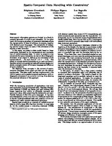
Complex models: Bayesian Examples in Italy

4495000

log(PM10), 95% C.I. upper

4495000

log(PM10)

4495000

log(PM10), 95% C.I. lower

statte

statte

690000

695000

700000

easting

lower 95% CI

(DSPSA-UNIROMA1)

670000

675000

680000

4490000 northing

talsanoarpa talsano

WIND_D N

W

+

E

S

685000

orsini

camuzzi peripato stadio carcere

ancona

3.1

690000

695000

easting

log PM10 map

700000

670000

3.1

4475000

gennarini

4470000

4475000 4470000

S

685000

16/12/2007 TEMP= 3.8 PRESS= 1014.32 HUMID= 53.62 RAIN= 0.4 RAD= 13.48 WV_MAX= 2.39

4485000

4485000

northing

4480000

4485000 4475000 4470000

E

3.05 archimede testa

3

680000

talsanoarpa talsano

N

+

3.1

5

675000

2.5

WIND_D

W

carcere

ancona

2.78

2.35

670000

16/12/2007 TEMP= 3.8 PRESS= 1014.32 HUMID= 53.62 RAIN= 0.4 RAD= 13.48 WV_MAX= 2.39

peripato stadio

2.45 gennarini

camuzzi

2.68

4480000

archimede orsini testa

2.95

paoloVI

3.0

carcere

ancona

2.8

northing

2.35 2.4stadio

3

3.05

3

peripato

2.74

camuzzi

2.45

paoloVI

2.72

testa

2.3

archimede orsini

2.5

7

2.66

paoloVI

2.62

4490000

2.

2.76

4490000

2.64

2.25

2.4

4480000

statte

2.5

16/12/2007 TEMP= 3.8 PRESS= 1014.32 HUMID= 53.62 RAIN= 0.4 RAD= 13.48 WV_MAX= 2.39

675000

680000

gennarini

3

2.95 talsanoarpa

talsano

WIND_D N

W

+

E

S

685000

690000

695000

700000

easting

upper 95% CI

TIES2009 Bologna

34 / 48

Complex models

Examples

Complex models estimation: the Bayesian framework advantages and disadvantages

In the Bayesian framework uncertainty can be rigourously and precisely evaluated

(DSPSA-UNIROMA1)

TIES2009 Bologna

35 / 48

Complex models

Examples

Complex models estimation: the Bayesian framework advantages and disadvantages

In the Bayesian framework uncertainty can be rigourously and precisely evaluated However the often huge computational effort required strongly limits these models use in practical application

(DSPSA-UNIROMA1)

TIES2009 Bologna

35 / 48

Complex models

Examples

Complex models estimation: the Bayesian framework advantages and disadvantages

In the Bayesian framework uncertainty can be rigourously and precisely evaluated However the often huge computational effort required strongly limits these models use in practical application In order to spread the use of this modeling approach it is necessary to develop easy to use software

(DSPSA-UNIROMA1)

TIES2009 Bologna

35 / 48

Composite models: multi-step procedures

Why multi-step?

Composite models: multi-step procedures

Often we are asked to produce efficient tools for decision makers, governmental agencies or other actors of the environmental management.

(DSPSA-UNIROMA1)

TIES2009 Bologna

36 / 48

Composite models: multi-step procedures

Why multi-step?

Composite models: multi-step procedures

Often we are asked to produce efficient tools for decision makers, governmental agencies or other actors of the environmental management. In these situations the computational issues pointed out before can seriously limit the use of complex models

(DSPSA-UNIROMA1)

TIES2009 Bologna

36 / 48

Composite models: multi-step procedures

Why multi-step?

Composite models: multi-step procedures

Often we are asked to produce efficient tools for decision makers, governmental agencies or other actors of the environmental management. In these situations the computational issues pointed out before can seriously limit the use of complex models However it is still possible to return rigorous (in a statistical sense) answers by combining several tools and models.

(DSPSA-UNIROMA1)

TIES2009 Bologna

36 / 48

Composite models: multi-step procedures

Why multi-step?

Composite models: multi-step procedures

Often we are asked to produce efficient tools for decision makers, governmental agencies or other actors of the environmental management. In these situations the computational issues pointed out before can seriously limit the use of complex models However it is still possible to return rigorous (in a statistical sense) answers by combining several tools and models. Usually this approach requires to sacrifice a precise and rigorous estimates uncertainty evaluation.

(DSPSA-UNIROMA1)

TIES2009 Bologna

36 / 48

Composite models: multi-step procedures

Examples

Composite models: multi-step procedures Jona Lasinio, Orasi, Divino, Conti (2007): Statistical protocol for the integration of buoy and WAve Model data, request from National Environmental Agency (now ISPRA) Focus on the correction of wave height measure produced by the ECMWF model using buoys measures from the Italian wave monitoring network (RON). Available data include wave height and direction opening several methodological issues.

(DSPSA-UNIROMA1)

TIES2009 Bologna

37 / 48

Composite models: multi-step procedures

Examples

Composite models: multi-step procedures

In order to produce a full hierarchical model in the study presented in Jona Lasinio et al. (2007) it would be appropriate to include directional data.

(DSPSA-UNIROMA1)

TIES2009 Bologna

38 / 48

Composite models: multi-step procedures

Examples

Composite models: multi-step procedures

In order to produce a full hierarchical model in the study presented in Jona Lasinio et al. (2007) it would be appropriate to include directional data. The solution found do not fully make use of the information on wave direction.

(DSPSA-UNIROMA1)

TIES2009 Bologna

38 / 48

Composite models: multi-step procedures

Examples

Composite models: multi-step procedures

In order to produce a full hierarchical model in the study presented in Jona Lasinio et al. (2007) it would be appropriate to include directional data. The solution found do not fully make use of the information on wave direction. The main issue becomes managing and modeling circular data.

(DSPSA-UNIROMA1)

TIES2009 Bologna

38 / 48

Composite models: multi-step procedures

Examples

Composite models: multi-step procedures

In order to produce a full hierarchical model in the study presented in Jona Lasinio et al. (2007) it would be appropriate to include directional data. The solution found do not fully make use of the information on wave direction. The main issue becomes managing and modeling circular data. In Ferrari et al (2008) and Ferrari (2009) preliminary ideas and some results have been presented while in this conference we described more recent results.

(DSPSA-UNIROMA1)

TIES2009 Bologna

38 / 48

Composite models: multi-step procedures

Examples

Composite models: multi-step procedures

In order to produce a full hierarchical model in the study presented in Jona Lasinio et al. (2007) it would be appropriate to include directional data. The solution found do not fully make use of the information on wave direction. The main issue becomes managing and modeling circular data. In Ferrari et al (2008) and Ferrari (2009) preliminary ideas and some results have been presented while in this conference we described more recent results. A full Bayesian model is proposed based on wrapped (on the circle) distributions. However computational difficulties are severe. We are working at making this approach practical for producing quick answers.

(DSPSA-UNIROMA1)

TIES2009 Bologna

38 / 48

Composite models: multi-step procedures

Examples

Composite models: multi-step procedures Pollice, Jona Lasinio (2009a, 2009b): Estimation of PM10 fields in the Taranto area request from the regional environmental Agency Area at high environmental risks due to the massive presence of industrial sites with elevated environmental impact activities. Large amount of missing data in the monitoring network, only one reliable source of meteo-covariate, different monitoring networks measurements.

(DSPSA-UNIROMA1)

TIES2009 Bologna

39 / 48

Conclusions

Concluding remarks

In this review I focused on continuous space discrete time processes and computational issues.

(DSPSA-UNIROMA1)

TIES2009 Bologna

40 / 48

Conclusions

Concluding remarks

In this review I focused on continuous space discrete time processes and computational issues. In this setting there is a strong need for computationally efficient solutions and software development.

(DSPSA-UNIROMA1)

TIES2009 Bologna

40 / 48

Conclusions

Concluding remarks

In this review I focused on continuous space discrete time processes and computational issues. In this setting there is a strong need for computationally efficient solutions and software development. In discrete space there exist some relevant results for Gaussian processes by Rue and coauthors (Rue, Held 2005, Rue, Martino 2006, Rue, Martino, Chopin 2009) that can be most likely extended to treat space-time phenomena to build computationally efficient tools.

(DSPSA-UNIROMA1)

TIES2009 Bologna

40 / 48

Conclusions

Concluding remarks: Future

I believe that there is going to be an increasing availability of space-time data that will continue to ask for new models and new software.

(DSPSA-UNIROMA1)

TIES2009 Bologna

41 / 48

Conclusions

Concluding remarks: Future

I believe that there is going to be an increasing availability of space-time data that will continue to ask for new models and new software. I especially appreciate the hierarchical models setting as it allows to easily include physical knowledge in the model.

(DSPSA-UNIROMA1)

TIES2009 Bologna

41 / 48

Conclusions

Concluding remarks: Future

I believe that there is going to be an increasing availability of space-time data that will continue to ask for new models and new software. I especially appreciate the hierarchical models setting as it allows to easily include physical knowledge in the model. As far as the huge amount of work I left out from this presentation, I can just ask the authors to forgive me: I had to make painful choices.

(DSPSA-UNIROMA1)

TIES2009 Bologna

41 / 48

Conclusions

Acknowledgements Special Thanks to Alessio Pollice, Daniela Cocchi and Alessandro Fass`o for the many ideas exchanges and the encouragement

Thanks for your attention (DSPSA-UNIROMA1)

TIES2009 Bologna

42 / 48

References by section

References: Introduction Adelfio G., Chiodi M., De Luca L., Luzio D., Vitale M. (2006a). Southern-Tyrrhenian seismicity in space-time-magnitude domain. Annals of Geophysics, vol. 49; p. 1245-1257, ISSN: 1593-5213. Adelfio G., Chiodi M., Luzio D., De Luca L. (2006b) Nonparametric clustering of seismic events. In: Data analysis classification and the forward search. ZANI, CERIOLI, VICHI, RIANI (EDITORS). p. 397-404, Heidelberg: Springer, ISBN/ISSN: 3-540-35977-X Adelfio G., Chiodi M. (2008a) Second-order diagnostic for space-time point process with application to seismic events. Environmetrics; p. 1-19, ISSN: 1180-4009, doi: 10.1002/env.961 Adelfio G., Schoenberg F. P. (2008b) Point process diagnostics based on weighted second-order statistics and their asymptotic properties. Annals of the Institute of Statistical Mathematics (in press). ISSN 0020-3157 (Print) 1572-9052 (Online). DOI: 10.1007/s10463-008-0177-1 Adelfio G., Ogata Y. (2008c) Hybrid kernel estimates of space-time earthquake occurrence rates using the Etas model. Annals of the Institute of Statistical Mathematics (in corso di stampa). Adelfio G., Chiodi M., Luzio D. (2008d). An algorythm for earthquake clustering based on maximum likelihood. In: Carlo Lauro; Francesco Palumbo; Michael Greenacre Editors. Data Analysis and Classification: From the exploratory to the confirmatory approach. p. 1-8. Heidelberg: Springer. Adelfio G., Chiodi M., Luzio D. (2008e). Comparison between nonparametric and parametric estimate of the conditional intensity function of a seismic space-time point process. In: Atti della XLIV Riunione Scientifica della Societ Italiana di Statistica (SIS). Universit della Calabria, 25-27 giugno 2008, p. 3-4, ISBN/ISSN: 978-88-6129-228-4 Chiodi M., Adelfio G. (2008). Semiparametric Estimation of conditional intensity functions for space-time processes. In: Atti della XLIV Riunione Scientifica della Societ Italiana di Statistica (SIS). Universit della Calabria, 25-27 giugno 2008, p. 1-2, ISBN/ISSN: 978-88-495-1656-2 Giunta G., Luzio D., Agosta F., Calo’ M., Di Trapani F., Giorgianni A., Oliveti E., Orioli S., Perniciaro M., Vitale M., Chiodi M., Adelfio G. (2008). An integrated approach to the relationships between tectonics and seismicity in northern Sicily and southern Tyrrhenian. Tectonophysics; p. 1-9, ISSN: 0040-1951, doi:10.1016/j.tecto.2008.09.031 Dreassi E (2003) A Space-Time analysis of the relationship between Material Deprivation and Mortality for Lung Cancer, Environmetrics, 14 (5), 511-521. Lagazio C., Dreassi E., Biggeri A. (2001) A Hierarchical Bayesian Model for the Analysis of Spatio-Temporal Variation in Disease Risk. Statistical Modelling, 1, 17-29 Lawson, A.B. (2008) Bayesian Disease Mapping: Hierarchical Modeling in Spatial Epidemiology. CRC Press. (DSPSA-UNIROMA1)

TIES2009 Bologna

43 / 48

References by section

References: Covariance Structures in historical order Shapiro, A. and Botha, J. D., (1991). Variogram fitting with a general class of conditionally nonnegative definite functions, Computational Statistics and Data Analysis, Elsevier, vol. 11(1), 87-96, Sampson P.D., Guttorp P. (1992) Nonparametric estimation of nonstationary spatial covariance structure. J Am Stat Assoc 87:108-119 Jones, R. H. and Y. Zhang (1997), Models for continuous stationary spacetime processes, in: T. G. Gregoire, D. R. Brillinger, P. J. Diggle, E. Russek-Cohen, W. G. Warren, R. D. Wolfinger (eds.), Modelling longitudinal and spatially correlated data, Springer Verlag, New York, NY, 289298. Stein,M. L. (1999), Interpolation of spatial data. Some theory of kriging, Springer-Verlag, New York, NY. Cressie, N. A. C. and C. Huang (1999), Classes of nonseparable, spatiotemporal stationary covariance functions, Journal of the American Statistical Association 94, 13301340. Brown, P. E., K˚ aresen, K. F., Roberts, G. O. and Tonellato, S. (2000), Blur-generated non-separable space-time models, Journal of the Royal Statistical Society Ser. B, 62, 847-860. Christakos, G. (2000), Modern spatiotemporal geostatistics, Oxford University Press, Oxford. De Cesare, L., D. Myers and D. Posa (2001), Product-sum covariance for spacetime modeling: an environmental application, Environmetrics 12, 1123. Christakos, G. (2002), On a deductive logic-based spatiotemporal random field theory, Probability Theory and Mathematical Statistics 66, 5465. Fuentes, M. (2002), Spectral methods for nonstationary spatial processes, Biometrika 89, 197210. Gneiting, T. (2002), Stationary covariance functions for spacetime data, Journal of the American Statistical Association 97, 590600. Ma, C. (2002), Spatio-temporal covariance functions generated by mixtures, Mathematical Geology 34, 965974.

(DSPSA-UNIROMA1)

TIES2009 Bologna

44 / 48

References by section

References: Covariance Structures in historical order

Fern´ andez-Casal, R., W. Gonzalez-Manteiga and M. Febrero-Bande (2003), Flexible spatio-temporal stationary variogram models, Statistics and Computing 13, 127136. Jun, M. and Stein, M. L. (2004a), Statistical comparison of observed and CMAQ modeled daily sulfate levels, Atmospheric Environment, 38, 4427-4436. Kolovos, A., G. Christakos, D. T. Hristopulos and M. L. Serre (2004), Methods for generating non-separable spatiotemporal covariance models with potential environmental applications, Advances in Water Resources 27, 815830 Stein, M. L. (2005), Spacetime covariance functions, Journal of the American Statistical Association 100, 310321 Porcu, E., Gregori, P., Mateu, J. (2006) Nonseparable stationary anisotropic spacetime covariance functions, Stoch. Environ. Res. Risk Assess, 21, 113-122 Porcu E., Mateu, J., Bevilacqua, M. (2007) Covariance functions that are stationary or nonstationary in space and stationary in time, Statistica Neerlandica, 61, 3: 358382 Yu,K. ,Mateu, J., Porcu E. (2007b) A kernel-based method for nonparametric estimation of variograms, Statistica Neerlandica 61, 2, 173197 Bevilacqua,M., Gaetan C., Mateu, J., Porcu, E. (2008) Estimating space and space-time covariance functions: a weighted composite likelihood approach Submitted Bruno F., Guttorp P., Sampson P.D., Cocchi D. (2008) A simple non-separable, non-stationary spatiotemporal model for ozone Environ Ecol Stat DOI 10.1007/s10651-008-0094-8

(DSPSA-UNIROMA1)

TIES2009 Bologna

45 / 48

References by section

References: Complex Models in historical order Christakos, G. (2000) Modern spatiotemporal geostatistics, Oxford University Press Stroud, J. R., Muller, P., and Sans` o, B. (2001), Dynamic Models for Spatiotemporal Data, Journal of the Royal Statistical Society, Series B, 63, 673689. Calder C.A. (2007) Dynamic factor process convolution models for multivariate spacetime data with application to air quality assessment Environ Ecol Stat (2007) 14:229247 DOI 10.1007/s10651-007-0019-y Cooley, D., D. Nychka, P. Naveau (2005). Bayesian spatial modeling of extreme precipitation return levels. Technical report, Geophysical Statistics Project, Boulder, CO. (published 2007 JASA 102: 824-840) Gelman, A., Pardoe, I., (2005). Bayesian measures of explained variance and pooling in multilevel (hierarchical) models. Technometrics 40 (2), 241-251. Gilleland, E. and Nychka, D. (2005) Statistical Models for Monitoring and Regulating Ground-level Ozone Environmetrics. 16, 535-546. Le, N. Z., Zidek, J. V. (2006). Statistical analysis of environmental space-time processes. New York: Springer. Sahu, S. K. and Mardia, K. V. (2005a) A Bayesian Kriged-Kalman model for short-term forecasting of air pollution levels. Journal of the Royal Statistical Society, Series C, Applied Statistics, 54, 223–244. Jona Lasinio, G., Sahu, S. K. and Mardia, K. V. (2005) Modeling rainfall data using a Bayesian Kriged-Kalman model. Sahu S.K., Jona Lasinio G., Orasi A., and Mardia, K.V. (2005b). A Comparison of Spatio-Temporal Bayesian Models for Reconstruction of Rainfall Fields in a Cloud Seeding Experiment. Journal of Mathematics and Statistics 1 (4), pp. 273–281 ISSN: 1549-3644. Sahu, S. K., Gelfand, A. E. and Holland, D. M. (2006) Spatio-temporal modeling of fine particulate matter. Journal of Agricultural, Biological, and Environmental Statistics. 11, 61–86.

(DSPSA-UNIROMA1)

TIES2009 Bologna

46 / 48

References by section

References: Complex Models in historical order

Cocchi D., Greco F., Trivisano C. (2007) Hierarchical space-time modelling of PM10 pollution Atmospheric Environment 41, 532-542 Gaetan C., Grigoletto M (2007). A hierarchical model for the analysis of spatial rainfall extremes. Journal of Agricultural Biological and Environmental Statistic, vol. 12; p. 434-449, ISSN: 1085-7117 Fass` o, A., Cameletti M. (2009a) A unified statistical approach for simulation, modeling, analysis and mapping of environmental data, Simulation: Transactions of the Society for Modeling and Simulation International, accepted.ISSN: 0037-5497. Fass` o, A., Cameletti M. (2009b) The EM algorithm in a distributed computing environment for modelling environmental space-time data, Environmental Modelling and Software, 24, pp. 1027-1035. Pollice, A., Jona Lasinio, G. (2009a). Two approaches to imputation and adjustment of air quality data from a composite monitoring network. Journal of Data Science,7, 43-59. Pollice A., Jona Lasinio G. (2009b) Spatiotemporal analysis of the PM10 concentration over the Taranto area, Environ Monit Assess DOI 10.1007/s10661-009-0786-z Sahu, S. K., Gelfand, A. E. and Holland, D. M. (2007) High Resolution Space-Time Ozone Modeling for Assessing Trends. Journal of the American Statistical Association. 102, 1221–1234. Sahu, S. K. and Nicolis, O. (2008) An evaluation of European air pollution regulations for particulate matter monitored from a heterogeneous network. To appear in Environmetrics.

(DSPSA-UNIROMA1)

TIES2009 Bologna

47 / 48

References by section

References: Conclusions

Rue, H. and Held, L. (2005). Gaussian Markov Random Fields: Theory and Applications, volume 104 of Monographs on Statistics and Applied Probability. Chapman and Hall, London. Rue H., Martino S. (2006) Approximate Bayesian Inference for Hierarchical Gaussian Markov Random Fields Models Rue H., Martino S., Chopin N. (2007) Approximate Bayesian inference for Latent Gaussian MOdels Using Integrated Nested Laplace Approximations,Tech Rep. accepted JRSSb (2009)

(DSPSA-UNIROMA1)

TIES2009 Bologna

48 / 48