Jul 9, 1997 - ranties, including, without limitation, the implied warranty of merchantability and fitness for a particular purpose. The TIMECENTER icon on the ...
Spatio-Temporal Database Support for Legacy Applications
Michael B¨ohlen, Christian S. Jensen, and Bjørn Skjellaug
July 9, 1997
TR-20
A T IME C ENTER Technical Report
Title
Spatio-Temporal Database Support for Legacy Applications
Copyright c 1997 Michael B¨ohlen, Christian S. Jensen, and Bjørn Skjellaug. All rights reserved.
Author(s) Publication History
Michael B¨ohlen, Christian S. Jensen, and Bjørn Skjellaug February 1997. Unpublished manuscript July 1997. A T IMEC ENTER Technical Report.
TIMECENTER Participants Aalborg University, Denmark Christian S. Jensen (codirector) Michael H. B¨ohlen Renato Busatto Heidi Gregersen Kristian Torp University of Arizona, USA Richard T. Snodgrass (codirector) Anindya Datta Sudha Ram Individual participants Curtis E. Dyreson, James Cook University, Australia Kwang W. Nam, Chungbuk National University, Korea Keun H. Ryu, Chungbuk National University, Korea Michael D. Soo, University of South Florida, USA Andreas Steiner, ETH Zurich, Switzerland Vassilis Tsotras, Polytechnic University, New York, USA Jef Wijsen, Vrije Universiteit Brussel, Belgium For additional information, see The T IMEC ENTER Homepage: URL:
Any software made available via T IMEC ENTER is provided “as is” and without any express or implied warranties, including, without limitation, the implied warranty of merchantability and fitness for a particular purpose. The T IMEC ENTER icon on the cover combines two “arrows.” These “arrows” are letters in the so-called Rune alphabet used one millennium ago by the Vikings, as well as by their precedessors and successors. The Rune alphabet (second phase) has 16 letters, all of which have angular shapes and lack horizontal lines because the primary storage medium was wood. Runes may also be found on jewelry, tools, and weapons and were perceived by many as having magic, hidden powers. The two Rune arrows in the icon denote “T” and “C,” respectively.
Abstract In areas such as finance, marketing, and property and resource management, many database applications manage spatio-temporal data. These applications typically run on top of a relational DBMS and manage spatio-temporal data either using the DBMS, which provides little support, or employ the services of a proprietary system that co-exists with the DBMS, but is separate from and not integrated with the DBMS. This wealth of applications may benefit substantially from built-in, integrated spatio-temporal DBMS support. Providing a foundation for such support is an important and substantial challenge. This paper initially defines technical requirements to a spatio-temporal DBMS aimed at protecting business investments in the existing legacy applications and at reusing personnel expertise. These requirements provide a foundation for making it economically feasible to migrate legacy applications to a spatio-temporal DBMS. The paper next presents the design of the core of a spatio-temporal extension to SQL–92, called STSQL, that satisfies the requirements. STSQL supports multiple temporal as well as spatial dimensions. Queries may “ignore” any dimension; this provides an important kind of upward compatibility with SQL–92. Queries may also view the tables in a dimensional fashion, where the DBMS provides so-called snapshot reducible query processing for each dimension. Finally, queries may view dimension attributes as if they are no different from other attributes.
1 Introduction A wide range of applications manage spatial, time-varying, or spatio-temporal data. Typically, CAD and GIS applications maintain huge volumes of spatio-temporal data, i.e., data that includes spatial extents, shapes, or locations of objects, and time-related versioning of data. Financial and record-keeping applications such as accounting, banking, personnel management, and medical records, manage large amounts of time-varying data. A common characteristic of applications such as these is that the semantics of spatial and time-varying data are the responsibility of and are encoded solely in the applications or some proprietary system [15, 22, 27]. That is, the semantics of the spatial and temporal dimensions, which are intrinsic properties of the data, are unknown to the underlying DBMS. Thus, spatio-temporal applications do not currently enjoy the built-in, integrated support that current DBMS’s already supply to less challenging applications. This paper addresses the challenges of providing spatio-temporal DBMS support to spatio-temporal data management applications. Legacy applications provide the toughest challenges: it should be possible to migrate them from their current inadequate platforms to a spatio-temporal DBMS. The database technology in the commercial market is not yet close to incorporating the necessary spatiotemporal capabilities. However, over the past decade or two, substantial research efforts in the areas of temporal and spatial data management have resulted in a substantial number of proposals for temporal and spatial data models and query languages (e.g., IXSQL [16], TempSQL [10], TSQL2 [26], ROSE Algebra [11], ParaSQL [6], Spatial SQL [8], and GEO System [20]). But, none of these proposals address the migration of legacy applications to a spatio-temporal DBMS. To be feasible, migrating legacy applications to a spatio-temporal DBMS must not require any substantial modifications to the legacy code for it to remain operational. The typically significant investments in the legacy applications must be protected. Stated more technically, a migration to a spatio-temporal DBMS has to protect existing data, application code, and personnel expertise. The paper defines a requirement aimed at guaranteeing that legacy application code, with its associated data, without modifications remains operational when migrated to the spatio-temporal DBMS. Another requirement aims at ensuring that new application code that exploits the new spatio-temporal support of the DBMS may co-exist harmoniously with the legacy code. Finally, a requirement aims at ensuring that programmers familiar with SQL–92 may start using the new features of the DBMS without a need for expensive training. Based on earlier work on a temporally extended SQL, termed ATSQL [4], we apply a set of more generic requirements to extend SQL–92 [17] to a spatio-temporal SQL, termed STSQL. STSQL supports the two 1
generic temporal aspects, valid time and transaction time, of database facts that record when facts are true in the modeled reality and when they are current in the database, respectively. STSQL may also associate the corresponding spatial aspects, valid space and transaction space, with facts, recording where facts are true and from where they are registered, respectively. The time and space values are recorded by timestamps and spacestamps that are associated with tuples as values of special attributes. STSQL also extends ATSQL in another major respect: ATSQL allows at most one valid time and one transaction time per table. STSQL permits multiple space and time dimensions for a single table. The paper is organized as follows. Following an introduction, in Section 2, of a case that will be used for illustration throughout, Section 3 defines three fundamental requirements to a spatio-temporal data model and query language. Section 4 proceeds by presenting the design of the spatio-temporal extension STSQL of SQL–92 that satisfies the requirements. At the end, Section 5 discusses related research, and Section 6 concludes the paper and outlines open research issues.
2 A Spatio-Temporal Data Management Application The case example presented here is based on an existing legacy planning and scheduling system (termed Ecoplan) used for forest management, specifically for long-term forest harvest scheduling based on ecological, recreational, and economical constraints [18]. While the system has four modules, we focus on the data module, which at present manages data in a loosely coupled fashion. Spatial data is stored in files and is managed by the module using proprietary data structures. The associated textual and numeric property data is managed by a relational DBMS. Using examples from this case, we will exemplify the design of a spatio-temporal relational data model step-by-step. To concisely illustrate the contributions of this paper, we have substantially simplified the system. We will thus assume that the system’s database contains three tables as shown in Figure 1. stands: st ID st 100 st 230 st 245 st 560
index high high low high
plans: specie pine birch birch spruce
planted 1935 1957 1946 1963
pl ID pl 29 pl 29 pl 29 pl 34
estates: st ID st 100 st 560 st 230 st 245
volume 2000 900 1500 400
ripe 2000 2000 2002 2010
es ID es 34 es 401 es 63 es 80
owner Paul Mary Mary Peter
Figure 1: A Case Example Database The stands table to the left captures data about regions that are homogeneous with respect to soil fertility (a so-called index), wood specie, and average age (set by the year the trees were planted). Thus, a tuple in stands records surveyed data about a forest region; the estates table to the right records the IDs of estates and their owners. Thus, an estate is a legal entity covering a geographical region, possibly including one or more forests. Finally, the plans table in the middle defines the harvest plans for stands, with each stand being associated with one or more plans (and vise versa), an estimated harvest volume in m3 for each stand, and an optimal harvest time (a so-called ripe year) of the stand. Thus, a plan of a stand is a calculation based on the stands data and specific scheduling parameters. Figure 2 illustrates the spatial locations of estates and stands, and it also indicates the plans of stands.
3 Migration Requirements This section defines and discusses three important requirements to a spatio-temporal data model and query language. While space and time are quite different aspects of data, the requirements are able to treat the two 2
st_560
st_230
pl_29
pl_29
es_63 es_401 st_245
es_34 stands
es_80
pl_34 st_100
estates
pl_29
Figure 2: Distribution of Estates and Stands with Related Plans aspects uniformly.
3.1 Overview When migrating to a new DBMS, it is desirable, or even essential, to protect existing investments in legacy application code and in programmer expertise. Informally stated, 1. all non-spatio-temporal legacy data is maintained by the new DBMS; 2. all non-spatio-temporal legacy code (i.e., queries and modifications) remains operational using the new DBMS, and it may access the same data as before; 3. skilled legacy system developers should with little effort be able to utilize a core subset of the added functionality in the spatio-temporal DBMS; and 4. the spatio-temporal DBMS should provide constructs to utilize the full potential of a spatio-temporal data model and query language. These requirements should be supported in concert by the data model and query language of a spatiotemporal DBMS (STDBMS). The next step is to make the requirements precise.
3.2 Compatibility Requirements The first two informal requirements above address upward compatibility issues, and are formally defined in the following. We will assume that a data model, M , is given by a query language component, QL, and a component of data structures, DS , manipulated by the query language. A data model captures the functionality of a DBMS that implements the data model. In the relational model, the most important user-level query language is SQL, and the table is the central data structure. With this convention, for a query language expression s and an associated database db, both legal elements of data model M = (DS; QL), define s(db) M as the result of applying s to db in data model M . With this notation, we can precisely describe the requirement to a new model that guarantees uninterrupted operation of all application code.
hh
ii
3
Definition 3.1 (upward compatibility—UC) Let two data models, M1 be given. Model M1 is upward compatible with model M2 iff
� 8db 2 DS db 2 DS , � 8s 2 QL s 2 QL , and � 8db 2 DS 8s 2 QL hhs 2
2(
1)
2
2( 2
2
2
2(
DS1 ; QL1 ) and M2 = (DS2; QL2 ),
=(
1)
2(
2
db2 )ii
2(
M2
=
hhs
db2 )ii
2(
M1
)).
Upward compatibility captures the conditions that need to be satisfied in order to allow a smooth transition from a current system, with data model M2 , to a new system, with data model M1 . The first two conditions imply that all existing databases and query expressions in the old system are also legal in the new DBMS. The last condition guarantees that all existing queries compute the same results in the new and the old DBMS. Thus, legacy application code remains operational, with no modifications necessary, when transitioning to the new DBMS. Upward compatibility ensures a smooth transition, but it does not guarantee a harmoneous co-existence between legacy and new application code. Friction between legacy and new code may occur when existing tables are altered to include new dimension attributes, i.e., spatial or temporal attributes. We thus formulate a requirement that existing application code on non-dimensional tables must continue to work unmodified when the tables are altered to become dimensional. Intuitively, the requirement is that a query q must return the same result on an associated snapshot database db as on the dimensional counterpart of the database, (db) (with operation adding dimensions to its argument database). Moreover, updates should not affect this.
D
D
Definition 3.2 (dimensional upward compatibility—DUC) Let a dimensional and a snapshot data model be given by Md = (DSd ; QLd ) and Ms = (DSs ; QLs ), respectively. Also, let be an operator that changes the type of a snapshot table to a dimensional table with the same explicit attributes. Next, let = u1 ; u2 ; : : : ; un (n 0) denote a sequence of update operations. With these definitions, model Md is dimensional upward compatible with model Ms iff
U
D
�
� M is upward compatible with M and � 8db 2 DS 8 U 8q 2 QL hhq U db ii s
d
s
s
(
(
s
s
(
s
( (
s
))
Ms
hhq U D db ii
=(
s
( (
(
s
)))
Md
)))).
The DUC requirement ensures that every legacy query computes the same result on a dimensionally extended database in the new, dimensional DBMS, as it would have done on the original database and evaluated in the old snapshot DBMS. To illustrate the requirements, consider the following three statements. We assume that the new STDBMS is in place and that it satisfies UC and DUC. > SELECT * FROM plans; > ALTER TABLE plans ADD harvest1 PERIOD AS VALID; > SELECT * FROM plans;
The first statement is an SQL–92 query issued on the legacy table, plans. Due to UC, it returns the same result as it did in the old DBMS. The next statement alters the plans table, by adding a valid-time dimension to indicate harvest periods of stands, perhaps because a new application needs this information about plans. The last statement is now on an extended table, but due to DUC it yields the same result as the first statement.
4
A UC evaluation is simply an evaluation that is identical to that of the legacy system, i.e., in this case an SQL–92 evaluation. A DUC evaluation, informally, simulates a non-dimensional database where only one state is maintained. To be more specific, a DUC evaluation on a temporal dimension considers simply the currently valid, or current, state and ignores past and future states. In queries, the argument tables are sliced as of the time now in each time dimension. Modifications, i.e., insertions, deletions, and updates are applied to and persists in the current state. Further details on the temporal aspects of DUC may be found elsewhere [2]. To achieve a DUC evaluation of queries on tables extended with one or more spatial dimension attributes, the approach is to simply ignore the spatial attributes—these attributes are eliminated using projections. Modification statements employ spatial default values and are discussed in further detail in Section 4.3. Having covered two compatibility requirements, the next step is to ensure that the spatio-temporal data model is a “natural” extension of the snapshot data model.
3.3 Reducibility Requirements To naturally generalize the snapshot relational model to a dimensional relational model, we adopt the view that a dimensional table simply is a collection of snapshot tables, with each snapshot table having an associated multi-dimensional point and containing all the snapshot tuples that have an associated multidimensional region that contains the point. To be more precise, we first define the notion of snapshot reducibility among data models. We will use r and r d for denoting a snapshot and a dimensional table, respectively. Similarly, db and dbd are sets d of snapshot and dimensional tables, respectively. The definition uses a dimensional slice operator, �pM ;M , which takes as arguments a dimensional table r d (in the data model M d ) and a dimensional point p. It returns a snapshot table r (in the data model M ) containing all tuples that are defined at point p. In other words, r consists of all tuples of r d , but without the dimensional attributes, whose associated (dimensional) region as defined by the combination of its dimensional attributes includes the point p. Definition 3.3 (snapshot reducibility) Let M = (DS; QL) be a snapshot relational data model, and let M d = (DS d ; QLd ) be a dimensional data model. Data model M d is snapshot reducible with respect to data model M if
8q 2 QL 9q 2 QL 8db 2 DS 8p (
d
d
(
d
d
(
�
(
d
M ;M p
q (db
(
d
d
q�
)) = (
d
M ;M p
db
(
d
)))))).
This concept of snapshot reducibility generalizes the similar concept from temporal databases in a straightforward manner [23]. The commutativity diagram in Figure 3 illustrates snapshot reducibility. The diagram states that for all query expressions q in the snapshot model (the bottom row), there must exist a query q d in the dimensional model (the top row) so that for all dbd and for all point arguments, the equality at the bottom right holds. Observe that q d being snapshot reducible with respect to q poses no syntactical restrictions on q d . It is thus possible for q d to be quite different from q , and q d might be very involved. This is undesirable, as we would like the dimensional model to be a straight-forward extension of the snapshot model. Consequently, we require that q d and q be syntactically similar. Definition 3.4 (syntactically similar snapshot-reducible extension—S-RED) [5] Let M = (DS; QL) be a snapshot data model, and let M d = (DS d ; QLd ) be a dimensional data model. Data model M d is a syntactically similar snapshot-reducible extension of model M if
� data model M
d
is snapshot reducible with respect to data model M , and 5
q
db
d
slice at p
�
d
M ;M p
?
db
(
d
- q (db )
d
d
d
slice at p
)
q
q(�
d
M ;M p
db
(
d
)) =
?
�
d
M ;M p
q (db
(
d
d
))
Figure 3: Snapshot Reducibility of Query q d with respect to Query q
� there exist two (possibly empty) strings, S
and S2 , such that each query q d in QLd that is snapshot reducible with respect to a query q in QL is syntactically identical to S1 qS2 . 1
If the two strings S1 and S2 are both the empty string, the extension is termed a syntactically identical snapshot reducible extension. The S-RED requirement makes it possible for the SQL–92 programmer to easily formulate spatiotemporal queries. To illustrate this, we first extend the estates and stands tables with two-dimensional valid-space attributes and then issue the following three spatio-temporal queries, which are explained next. (Remember that we earlier extended the plans table with a valid time attribute.) > ALTER TABLE estates ADD es_area 2D_REGION AS VALID; > ALTER TABLE stands ADD st_area 2D_REGION AS VALID; > SEQUENCED (es_area) 2D_REGION ’Sherwood_Forest’ SELECT * FROM estates; > SEQUENCED (harvest1) PERIOD ’1996’ SELECT plans.st_ID FROM plans; > SEQUENCED (es_area st_area) AS area SELECT es_ID, st_ID FROM estates, stands;
Note that the queries have an SQL–92 core and are prepended with a SEQUENCED string. The string, termed a flag, indicates how to handle the dimension attributes in the queries and also restricts the qualifying tuples based on the values of their dimension attributes. Flags in STSQL is an important topic of the next section. The first statement returns all tuples of estates, with the restriction that the es area attribute of a qualifying tuple must overlap with the 2D REGION denoted by Sherwood Forest. The second statement finds stands that were harvested in 1996. The third statements retrieves estate and stand pairs with intersecting areas, along with their common areas. It thus computes a spatial Cartesian product. Imagine that all spatial values for estates and stands, shown in Figure 2, are stored in the database in Figure 1. Then the result of this query contains these two tuples:
hes 34, st 245, reges 34 \ regst 245 i hes 80, st 245, reges 80 \ regst 245 i This result is arrived at by computing the query in a point-by-point fashion, as indicated by the presence of the SEQUENCED flag. More specifically, for every point in space for which both an estate and a stand tuple is space-valid, a tuple with the pair of IDs of the estate and stand contributes to the result, and STSQL also includes the space-valid point with the result. Upon finding all snapshot pairs of IDs and associated space 6
points that contribute to the result, tuples with identical ID pairs are replaced by a single tuple that has the same ID values and stores as an attribute area the region corresponding to the union of all the tuples’ space points. (Here, we assume that the data type used for spatial regions, i.e., the data type of area is capable of representing any union of points in space. If this is not the case, several tuples may be needed for capturing the spatial region of a pair of IDs.) This way, a pair of IDs in the result has associated as attribute area the intersection of the particular tuples’ estate and stand regions, as stored in es area and st area. Thus, one stand may join with more than one estate and one estate may join with more than one stand. In summary, a snapshot reducible query generalizes a snapshot query by reducing argument dimensional tables to point-indexed snapshot tables, then computes the corresponding snapshot query on those snapshot tables, and finally “unions” the snapshot results to achieve a dimensional result table. Our use of the period data type for time dimensions limits the extent to which tuples with identical non-dimensional attribute values, termed value equivalent [13], may be “unioned,” termed coalesced [13]. Specifically, two tuples may only be coalesced into one if their time dimensions overlap. The main characteristic of snapshotreducible evaluation is its point-based nature, where dimensional tables may be seen as indexed sequences of snapshot tables. Hence, the key word SEQUENCED. A spatio-temporal query language should also provide queries that have no counterparts in the snapshot query language. That topic is considered next.
3.4 Beyond Reducibility Reducible STSQL queries perform computations on the dimension attributes as specified by reducibility and by the SQL–92 queries they reduce to. The advantage is that it is easy to immediately write a wide range of dimensional queries that perform potentially complex manipulation of dimension attributes. However, reducible queries also have limitations. Indeed, many reasonable and useful dimensional queries cannot be specified as reducible generalizations of snapshot queries. There is a need for the ability to specify queries where no processing of the dimension attributes is hard-wired into the data model, but where instead the programmer has complete control over the manipulation of the dimension attributes. The approach we adopt is to make it possible to specify in the flag of a statement that dimension attributes should be considered as regular attributes, with no built-in semantics in the query language. In addition, we provide a range of predicates and function that operate on the data types of the dimension attributes. This gives the programmer full control over the dimension attributes. For example, non-reducible queries may relate database states that apply to different points in multi-dimensional space. For this reason, we use the key word NONSEQUENCED to indicate dimension attributes that should be treated as regular attributes in a query. An example follows. > NONSEQUENCED (es_area st_area) SELECT e.es_ID, s.st_ID, INTERSECT(es_area, st_area) AS area FROM estates e, stands s WHERE es_area OVERLAPS st_area;
This query is similar to the last reducible query given in Section 3.3. The flag specifies that the two dimension attributes es area and st area of estates and stands, respectively, should be treated as regular attributes in the query. The result of the query is a snapshot table with the attributes specified in the SELECT clause. Since there is no built-in dimension processing, an explicit OVERLAPS predicate is necessary in the WHERE clause to obtain the effect of the reducible query from earlier. Note that, while this example allows us to replace the sequenced query with a nonsequenced one, this is not feasible in general.
7
3.5 Summary We have introduced three ways of handling dimension attributes in spatio-temporal tables. Dimension attributes that are not mentioned in the flag of a query language statement are “ignored,” or treated consistently with the dimension upward compatibility requirement. If the key word SEQUENCED is used for dimension attributes, they are treated as implicit dimensions of data, and the statement is evaluated with semantics that meet the snapshot reducibility requirement. This provides built-in spatio-temporal query processing. Finally, if the key word NONSEQUENCED is used for dimension attributes in the flag of a statement, the dimension attributes are treated as regular attributes. This provides maximum flexibility in writing spatiotemporal queries.
4 STSQL design This section discusses the design of a spatio-temporal extension to SQL–92 based on the requirements and evaluation modes discussed in Section 3. We briefly discuss the new datatypes of STSQL, then explore in more detail its syntax and semantics. It is an important characteristics of STSQL that it seamlessly extends SQL–92 in that it prepends SQL– 92 statements with an optional flag. If this flag is omitted, legacy SQL–92 statements result. This approach makes the semantics of STSQL relatively easy to define in terms of SQL–92 and to understand for someone familiar with SQL–92. When formulating a query, the core SQL–92 statement can be formulated as usual— not considering the dimensions. The flags may then be added to handle the dimensions as desired.
4.1 Space and Time Data Types The initial step in the design of STSQL is to introduce new datatypes that capture time and space values. For time values STSQL uses anchored time periods. Spatial values are unions of regions. Regions are either defined over 1-, 2-, or 3-dimensional spatial domains. The corresponding datatypes are PERIOD, 1D REGION, 2D REGION and 3D REGION, respectively. A further specialization of the region datatype would lead to points, (poly-)lines, rings, and polygons. In this paper, the number of different region data types and their individual characteristics are of minor importance (the interested reader is referred to, e.g., G¨uting [11] for more details about a variety of spatial data types). The new data types must be accompanied by predicates and functions that operate on them. Again, the specific choice and number of these is not important for the contribution of this paper, so we simply give a list of names and brief informal definitions of some useful, representative predicates and functions. name BEGIN/END MEETS OVERLAPS CONTAINS PRECEDES INTERSECT DURATION AREA
definition timestamp’s start/end time adjacent/neighbors sharing some instants/points one within the other one strict earlier than the other shared period/region length of period in specified units number of square units
domain period period/region period/region period/region period period/region period region
value time instant boolean boolean boolean boolean period/region a number a number
The predicates for periods and regions should be well known to those familiar with, e.g., Allen’s interval logic [1] and Egenhofer and Franzosa’s point-set topological spatial relations [9].
8
4.2 Dimensional Tables and Databases The next step is to make tables dimensional, in order to provide a basis for built-in dimensional support for modifications and queries in the query language. The data types introduced in the previous section are utilized. As a precursor to creating actual dimensional tables using the data types, we note that the data types, like any other SQL–92 data types, may be employed for defining domains of attributes that are in principle no different from regular attributes. Including such attributes in a table does not render the table dimensional; rather, the table is a regular table that includes regular attributes, some or all of which happen to be of type PERIOD, 1D REGION, 2D REGION, or 3D REGION. The DBMS attaches no special semantics to these attributes. To provide built-in dimensional support, e.g., dimensional upward compatibility and snapshot reducibility, it is necessary to be able to designate certain time or space valued attributes as special dimensional attributes. Tables with such attributes are then dimensional tables. In STSQL, dimensional tables may have any number of dimensional attributes, and each dimension attribute may be of any of the four new time and space types introduced in Section 4.1. In addition, a dimension attribute is specified as either a VALID or a TRANSACTION attribute. Combining the options for defining dimension attributes, we obtain four conceptually different types of dimension attributes. With d att being the name of a dimension attribute, the four types are as follows (where x denotes 1, 2, or 3). d d d d
att att att att
PERIOD AS PERIOD AS xD REGION xD REGION
VALID TRANSACTION AS VALID AS TRANSACTION
In typical use, a dimension value of a tuple is associated with the tuple as a whole. In the first type, d att then records when some temporal aspect of the information recorded by the (non-dimensional) attributes of the tuple as a whole is true, or valid, in the mini-world. For example, we have previously added a harvest1 attribute to the plans table, recording the harvest period for a plan. While with the first type above, we record when some temporal aspect of a tuple is valid, the second type records when a tuple is current in the table, or, equivalently, when we believed in the information recorded by the tuple. This transaction-time aspect of a tuple is important in applications that require accountability or traceability of database modifications. Where valid-time values are determined by the mini-world modeled by the database, the transaction-time values are determined by the modification activity on the database. The two last types replace time with space. The first of these types records some spatial aspect of a tuple. For example, we have previously added the attribute es area 2D REGION AS VALID to the estates table. This dimensional attribute is intended to record the geographic areas of individual estates. We have also added a dimensional st area attribute to the stands table for recording the specific regions of forests that are surveyed and found homogeneous with respect to certain parameters. Transaction-time attributes were used for recording when tuples are current in a table. The last type of dimension attribute records where a tuple was recorded. Notationally, we term this a transaction-space attribute. In contrast to most spatial and temporal models, STSQL permits multi-dimensional tables where a single table may have any number of dimension attributes of any of the types explored above. This added generality is useful for many purposes. Several valid-time attributes are useful, e.g., when the information of a tuple is true in several different (possible) worlds. For example, different historians, archeologists, or interest groups may possess different, competing world views, all of which could be represented in a single table. 9
Several VALID-type attributes may also record different temporal aspects of a tuple. For example, the plans table previously presented, had a VALID attribute harvest1 recording when a stand is supposed to be harvested. We can also add a new VALID attribute denoting when the textual property data about a plan for a stand are valid. Certainly, these two attributes record different aspects of a plan. We may also add a VALID attribute recording an alternative harvest period that denotes a harvest period of a stand calculated using a different method and different parameters. The resulting two harvest attributes reflect different (possible) worlds. Reasons for recording multiple transaction-time attributes have been explored elsewhere [14]. The choice of how to use multiple valid and transaction times is up to each specific application. Considering space instead of time, it is equally easy to envision uses of multiple dimension attributes: The multiple-worlds argument applies equally well to space, and tuples may have several different kinds of spatial aspects. Couclelis discusses issues related to these [7]. Furthermore, several transaction-space attributes may simply record that (parts of) a tuple are recorded jointly from several locations. In summary, we have added multiple space and time dimensions to tables, thereby obtaining the semantics necessary to enable dimensional semantics to be built into modifications and queries. The next step is to explore the management of databases with multi-dimensional tables.
4.3 STSQL Statements This section presents the core of STSQL. EBNF syntax is given for the central extensions to SQL–92. Examples from the forest management application are used for illustrating the semantic properties of STSQL. 4.3.1
Dimensional Default Values
In various situations, SQL–92 inserts a default value whenever a regular attribute value is missing. This occurs if an insert statement lacks a value, if a tuple referenced by a foreign key is deleted, or if an alter statement adds an attribute to a table. In all these cases, SQL–92 resorts to a user-defined default value or, if none is specified, to the system-default, NULL. STSQL adheres to this approach whenever reasonably possible, but there are also situations where STSQL has to extend this approach in order to get the intended semantics for the dimensions of tables, especially where DUC evaluation is involved. For example, the transaction time of inserted tuples must extend to the current time, and legacy SQL–92 statements are evaluated on only the current database state, as discussed briefly in Section 3.1 [2]. For time dimensions, the implicit handling of timestamps has been investigated carefully [2]. DUC query expressions are evaluated only on tuples with valid and transaction times that overlap with now. DUC modification statements are slightly more complicated. Common to all DUC modification statements is that they affect current and future data only. Thus, tuples inserted by SQL–92 statements get valid and transaction time periods from the current time until now, whereas SQL–92 deletions set the end times of periods of tuples to be deleted to the current time, making the tuples invisible to future SQL–92 queries. In contrast to the temporal dimensions there are no obvious default values for spatial dimensions. One possible value would be to use some notion of “current” location, but it is unclear how well this choice would make it possible to reflect real-world semantics. We therefore have decided to let DUC queries ignore spatial dimensions. This is consistent with how spatial dimensions are handled when spatial values are captured using explicit attributes: if such attributes are not mentioned explicitly (e.g., in the SELECT clause), they are simply ignored. This choice for handling spatial dimensions in queries poses no restrictions on our choices for handling legacy modifications. Legacy SQL–92 modifications set the transaction space to the location where the
10
transaction is issued, i.e., the current location. For valid space, a legacy modification inserts a default spatial value, i.e., either a user-defined default or the system default, NULL. These choices are compatible with STSQL being dimensional upward compatible with SQL–92. The issues are exemplified and discussed further in the following. 4.3.2
Alter and Create Statements
Legacy tables can be extended with spatial and temporal dimensions. For example, the following statements extend the tables from our case with further dimensions. > > > > > > >
ALTER ALTER ALTER ALTER ALTER ALTER ALTER
TABLE TABLE TABLE TABLE TABLE TABLE TABLE
estates estates plans plans stands stands stands
ADD ADD ADD ADD ADD ADD ADD
es_vt es_tt pl_vt harvest2 survey st_vt st_tt
PERIOD AS PERIOD AS PERIOD AS PERIOD AS PERIOD; PERIOD AS PERIOD AS
VALID; TRANSACTION; VALID; VALID; VALID; TRANSACTION;
These statements make estates a three-dimensional table with a transaction-time, a valid-time, and a valid-space dimension (cf. Section 3). The plans table becomes a three-dimensional valid-time table. The stands table is altered to include a valid-time dimension, a transaction-time dimension, and a user-defined attribute, the latter denoting the period during which a stand is surveyed. Note the difference between survey and st vt. The former is not a dimension and, therefore, not covered by upward compatibility, dimensional upward compatibility, or reducibility. Similar syntactic extensions apply to create statements. As an example, we next define a table that keeps track of owners of estates. > CREATE TABLE people ( name VARCHAR(40), street_addr VARCHAR(60), phone VARCHAR(10), vt PERIOD AS VALID, tt PERIOD AS TRANSACTION); 4.3.3
Queries, Flags and Dimension Identifiers
Next, we explore dimensional queries. All sample queries are evaluated on the tables shown in Figure 4. In order to understand the queries and modifications, it is essential to understand the semantics associated with these tables. We discuss each table in turn. 1. The stands table models the (surveyed and analyzed) status of stands. For each stand we record, e.g., the specie of the stand’s dominant tree population, the soil fertility of the stand (i.e., the index), the stand’s location, and a period of validity. A transaction time is used to retain a record of modifications. In stand st 100, pines have good growing conditions, i.e., high soil fertility. They were planted in 1935 and the stand was surveyed between 1984 and 1986. The stand location is the region regst 100 . The information has been valid since 1989, but was first recorded 1996. 2. The estates table records for each estate its owner, the validity period of the ownership, and the area that it covers. A transaction time is used to record modifications. 11
stands st ID index st 100 high st 230 high st 245 low st 560 high
specie pine birch birch spruce
planted 1935 1957 1946 1963
estates es ID owner es 34 Paul es 63 Mary es 80 Peter es 401 Mary es 80 Peter es 401 Mary es 100 Tom plans pl ID pl 29 pl 29 pl 29 pl 34 pl 35
st ID st 100 st 560 st 230 st 245 st 245
volume 2000 900 1500 400 500
survey 1984-1986 1984-1986 1984-1986 1984-1986
es area reges 34 reges 63 reges 80 reges 401 reges 80 reges 401 reges 100
ripe 2000 2000 2002 2010 2011
st vt 1989-now 1989-now 1989-now 1989-now
es vt 1995-now 1996-now 1996-now 1996-now 1996-1999 1996-1999 2000-now
pl vt 1996-now 1996-now 1996-now 1995-1996 1997-now
st tt 1996-now 1996-now 1996-now 1996-now
st area regst 100 regst 230 regst 245 regst 560
es tt 1994-now 1996-now 1995-1996 1995-1996 1997-now 1997-now 1997-now
harvest1 1998-2000 1999-2001 2000-2002 2009-2011 2010-2012
harvest2 1999-2004 2001-2003 2005-2008 2009-2011 2010-2012
Figure 4: The Spatio-Temporal Example Database During 1995 and 1996, it was recorded that estate es 80, covering area reges 80 , was owned by Peter from 1996 onwards. Similarly, it was recorded that estate es 401, covering area reges 401 , is owned by Mary from 1996 onwards. In 1997, Mary and Peter agreed to sell their estates es 401 and es 80, respectively, to Tom, effective as of year 2000. Tom’s estate will then cover the area reges 100 , which is the union of the two previous estates. 3. The plans table records how stands are cultivated. For each stand, we record the volume to be harvested and the ripe year. Each plan has two harvest periods, calculated according to different scheduling methods that emphasize some growth conditions differently, e.g., according to soil fertility, climate, etc. Plan pl 34 schedules stand st 245 to be harvested from 2009 to 2011. The expected harvest volume is 400m3 , and the ripe year is 2010. At some point, plan pl 34 for stand st 245 is superseded by plan pl 35. The new plan postpones the harvest period to 2010–2012 because, due to new climate estimates, the new expected ripe year has moved to 2011. The new expected harvest volume is 500 m3 . The syntactic extensions to SQL–92 that are needed to formulate spatio-temporal statements are relatively few. The flag is the central novel construct and is used to indicate the desired evaluation mode(s) (cf. Section 2). Flags are placed in front of SQL statements and indicate whether the statements have to be evaluated sequentially and/or non-sequentially. Additionally, it is possible to express domain restrictions and range specifications. 12
The following EBNF defines the syntax of flag. The is the standard’s production for the SELECT statement [17]. ::= flags [ ] flags ::= [ flag { "AND" flag } | range_spec { "AND" range_spec } ] flag ::= modifier dimensions [ domain_constant ][ range_spec ] range_spec ::= "SET" dim_datatype range_expression modifier ::= "SEQUENCED" | "NONSEQUENCED" dimensions ::= "(" column_reference { column_reference } ")" [ "AS" ] dim_datatype ::= PERIOD | 1D_REGION | 2D_REGION | 3D_REGION
The dimension(s) that a particular flag modifier applies to is (are) given by the non-terminal dimensions and have to follow the sequenced or nonsequenced modifier. Because of the multi-dimensional nature of STSQL, dimensions have to be named explicitly—unlike in frameworks with a fixed number of dimensions, this information cannot be inferred automatically. To be meaningful, a sequenced evaluation must apply to precisely one dimension from each argument table in the SQL statement. This requirement reflects the fact that a flag (and thus a sequenced evaluation) applies to an entire statement. In general, no meaningful semantics can be given to sequenced statements with tables that do not participate in the sequenced evaluation. Note that derived table expressions (i.e., table expressions in the from clause) start a new scope whereas subqueries, in the where clause, do not start a new scope. It should also be clear that the dimension types that take part in a sequenced evaluation must be homogeneous. Sequenced semantics are not meaningful when combining valid time and valid space or transaction time and valid time because of the different semantics associated with the respective dimensions. When formulating queries on dimensional tables, it is advantageous to proceed in several steps. Initially, all dimensions are ignored and the core STSQL query, typically an SQL–92 query, is formulated. The next steps concern the formulation of the query’s flag. For each dimension of each table in the query, we must determine and express in the flag the dimension’s use in the query. First, we determine what dimensions should be evaluated with sequenced semantics. Each occurrence of the SEQUENCED keyword requires the participation of exactly one dimension from each table. Second, we determine which dimensions are to be given NONSEQUENCED semantics. This semantics is chosen if we want to formulate user-defined predicates (e.g., CONTAINS) on the attribute or if we want to override DUC consistent semantics, which is the semantics given to dimension attributes not mentioned in the flag. In the sequel, a set of example queries are employed to illustrate the concepts introduced above and the formulation of queries in STSQL. Query Q1 For each stand that is ripe in 2000, determine its harvest periods. This query requires us to join the stands and the plans tables. We use a sequenced join over the valid times to associate stands with relevant plans only. Next, we are only interested in the stands table as best known as of now, i.e., we restrict the transaction time to overlap now. This is exactly the semantics provided by DUC and we therefore do not specify any flag for st tt. The location of a stand is not relevant and, thus, must be disregarded. This semantics is supported by DUC, which means that no flag for st area has to be specified. Finally, we want to retrieve (and handle) the harvest periods like regular attributes. This is achieved by specifying a nonsequential flag for these dimensions.
13
> SEQUENCED (st_vt, pl_vt) AS vt AND NONSEQUENCED (harvest1, harvest2) SELECT st.st_ID, specie, index, harvest1, harvest2 FROM stands st, plans pl WHERE pl.st_ID = st.st_ID AND st.ripe = 2000; st.st_ID specie index harvest1 harvest2 vt ------------------------------------------------------st_100 pine high 1998-2000 1999-2004 1996-now st_560 spruce high 1999-2001 2000-2003 1996-now
Query Q2 Determine all stands that did not change status for more than 5 years, together with the corresponding estate(s). This query requires us to sequentially join a) the locations of stands and estates and b) the valid times of both tables. Additionally, we have to specify a where clause condition that captures the user-defined restriction on the valid time of stands. Because we are only interested in the table contents as best known as of now we restrict the transaction times to overlap now. This is exactly the semantics provided by DUC and we therefore do not specify any flag for the transaction times. > SEQUENCED (st_area, es_area) AS st_es_area AND SEQUENCED (st_vt, es_vt) AS st_es_vt SELECT st_ID, es_ID FROM stands, estates WHERE DURATION(st_vt, YEAR) > 5;
Query Q3 For all stands, determine when the two harvest periods are scheduled contemporarily. Searching for contemporary occurrences (i.e., at every instant the harvest periods overlap) hints at sequenced semantics. In this case, we have to self-join the stands table, thereby sequentially joining harvest1 and harvest2. Note that a nonsequential semantics has to be specified for those harvest periods we are not interested in, i.e., harvest2 for pl1 and harvest1 for pl2, respectively. We have to do so to prevent a DUC-consistent evaluation. Such an evaluation would restrict the times of the respective harvest periods to the current time, which is clearly not what we want. > SEQUENCED (pl1.harvest1, pl2.harvest2) AS agreed_harvest AND NONSEQUENCED (pl1.harvest2, pl2.harvest1) SELECT pl1.st_ID FROM plans pl1, plans pl2 WHERE pl1.st_ID = pl2.st_ID;
Query Q3’ The astute reader might wonder why we do not simply state an explicit selection predicate that requires the harvest periods to overlap. This, of course, is also possible. Query Q3’ produces the same result as Query Q3, the only difference being that agreed harvest is a dimension attribute in the former and a regular attribute in the lattter. > NONSEQUENCED (harvest1, harvest2) SELECT st_ID, INTERSECT(harvest1, harvest2) AS agreed_harvest FROM plans WHERE harvest1 OVERLAPS harvest2;
Query Q3’ is shorter, and without an enhanced query optimiser we can expect this query to evaluate faster than Q3. However, there is an important difference between the two queries. This becomes clear if we consider a (slight) variation of the original query. 14
Query Q4 For all stands, determine when the first harvest period is ongoing while the second is not. The only difference from Q3 is that we are not looking for contemporary occurrences of harvest1 and harvest2, but for exclusive occurrences of harvest1. Our first solution scales up nicely. The flags remain exactly the same. We only have to change the SQL statement to specify a negation rather than a join. > SEQUENCED (pl1.harvest1, pl2.harvest2) AS light_harvest AND NONSEQUENCED (pl1.harvest2, pl2.harvest1) SELECT pl1.st_ID FROM plans pl1 WHERE pl1.st_ID NOT IN ( SELECT pl2.st_ID FROM plans pl2 );
The formulation of this query becomes much more complex with the second approach, i.e., the Q3’ approach. Depending on the exact data, the representation of timestamps, and the functions on timestamps, it can become exceedingly difficult to formulate queries with this approach. This indicates that built-in sequential processing is both powerful and user-friendly. Thus having explored queries, we turn our attention to modification statements. 4.3.4
Modification Statements
The EBNF of STSQL modifications is shown below. It is similar to that of SQL–92, the difference being that statements can be prepended with flags.
Statements with an empty flags clause are either UC or DUC modifications. Otherwise, the modification is SEQUENCED or NONSEQUENCED, possibly restricted by a range spec clause. In the following, examples of inserts and updates in our case are used for illustrating how STSQL behaves for various types of statements. First, some DUC statements are issued. A newly surveyed forest region has got its data analyzed and its plan scheduled. A legacy application issues the following statements on January 15, 1997. > INSERT INTO stands VALUES (’st_562’, ’medium’, ’spruce’, 1952, 1996-1997); > INSERT INTO plans VALUES (’pl_34’, ’st_562’, 9000, 2011); > COMMIT;
Since the stands and plans tables both are dimensional, the DUC evaluations of these statements provide default values for the dimension attributes of the respective tables. The following two tuples result from evaluating the two statements, i.e., the new tuples are as follows.
hst 252, medium, spruce, 1952, 1996 ? 1997, 1997 ? hpl 34, st 562, 9000, 2011, 1997 ? 1997 ? now;
1997 ? now; NULLi 1997 ? nowi
now;
now;
Note that DUC evaluations implicitly add values for unspecified dimensions, i.e., for the valid times, the transaction time, the area, and the two harvest periods. While it has been shown that in uni- and bitemporal tables, it is reasonable to timestamp “from the current time onwards,” this is less obvious in multi-temporal 15
frameworks. In our example, it certainly makes sense to apply this default to st vt, st tt, and pl vt. However, this makes less sense for the harvest periods. On the other hand, we have no other value that is clearly superior. (This illustrates that dimensional upward compatibility is limited in scope when it comes to the interpretation of timestamps, which is not surprising.) The st area dimension for stands is set to NULL because no user default was specified when the dimension was added. A range specification can be used to insert past, present, or future data. > SET es_vt PERIOD ’1956-1986’ AND SET es_area 2D_REGION ’reg_es_63’ INSERT INTO estates VALUES (’es_63’, ’Jim’); > COMMIT;
Recall that a range specification is used to set/add dimension values in query, insert, or update statements. In simple modification statements, it is also possible to use standard techniques to set dimension values (e.g., add the range expressions to the value list). > INSERT INTO estates VALUES (’es_63’, ’Jim’, ’reg_es_63’, ’1956-1986’); > COMMIT;
While possible, this type of insertion is not recommended because the position of the dimension attributes has to be taken into consideration (the same problem exist for standard attributes in SQL–92) and because this format is inapplicable if the values to be inserted are defined in terms of an SQL query expression. Next, it is discovered that Paul’s correct name is Jean Paul. The wrong information is corrected independently of time and space, i.e., with a nonsequenced statement. > NONSEQUENCED (es_vt, es_area) UPDATE estates SET owner = ’Jean Paul’ WHERE owner = ’Paul’; > COMMIT;
Internally, the transaction time end of the current tuple, i.e., the tuple with name Paul, is set to the current time and a new tuple with name Jean Paul is inserted.
hes 34, Paul, reges 34 1995 ? hes 34, Jean Paul, reges 34 1995 ? ;
now;
;
1994 ? 1996i 1997 ? nowi
now;
Finally, we give a statement that postpones the average planting time by two years for stands located within estate es 63. > SEQUENCED (st_area, es_area) UPDATE stands SET planted = planted + INTERVAL ’2 YEAR’ WHERE EXISTS ( SELECT * FROM estates WHERE es_ID = ’es_63’ ); > COMMIT;
Note that all STSQL modification examples include core SQL statements. Thus, if the STSQL-specific prepended strings are removed, the core of the statements are all legal SQL statements. This yields a userfriendly query language. The above SQL statements, that could be part of a legacy application, are easily turned into spatio-temporal statements. This means that it is possible to easily extend legacy applications to become spatio-temporal, which is beyond simply permitting legacy applications to co-exist with new spatio-temporal applications. 16
5 Related Work The migration requirements that dictate the general properties of STSQL were originally developed in the context of bitemporal tables, i.e., tables supporting, at most, one transaction time and one valid time [2]. STSQL supports multiple valid- and transaction-time and multiple valid- and transaction-space attributes in a single dimensional table. We are aware of no other models with this property. Among the few spatio-temporal data models that exist, ParaSQL [6] may be the closest relative of STSQL. Being based on an attribute-value stamped data model, ParaSQL differs substantially from STSQL; apart from upward compatibility, it is our contention that it does not satisfy any of the migration requirements. Within temporal databases, ATSQL [4] and proposed additions to the SQL/Temporal part of the SQL3 standard [24, 25] support bitemporal tables and also satisfy the migration requirements. STSQL may be seen as a generalization of these languages, its closest temporal relatives. Considering spatial data models, we have found no data models that provide migration support beyond upward compatibility. The SQL-based languages GEOQL [19], PSQL [21], KGIS [12] and Spatial SQL [8] preserve the non-dimensional SQL and satisfy UC, and they define explicit extensions to the SQL select statement for the handling of spatial values. KGIS and Spatial SQL also define, outside SQL, other language constructs to augment the spatial capabilities of their models and languages.
6 Conclusion and Future Research This paper has investigated how existing database applications using a conventional SQL–92-based DBMS may be migrated to a spatio-temporal DBMS without changing the application code; it has investigated how new spatio-temporal applications may be added without affecting the existing applications; and it has investigated how to reuse programmer expertise by designing the spatio-temporal SQL carefully. A spatio-temporal extension to SQL–92, termed STSQL, that aims at satisfying the above requirements, while providing built-in data management support for spatio-temporal data, has been explored. No other spatio-temporal language satisfies all the requirements. Within temporal databases, two bitemporal query languages satisfy the requirements; unlike these two languages, STSQL supports an arbitrary number of temporal and spatial attributes with built-in support in the query language. This paper presents the initial design of the core of STSQL, and in doing so, it touches upon a variety of language facilities. However, further formalizations of the language, beyond the informal semantics give here, is warranted. Perhaps most prominently, the semantics of spatio-temporal modifications have yet to be determined in full, and then specified. In this paper, we have chosen one reasonable semantics for DUC statements, but in a multidimensional framework, there appears to be several reasonable semantics for these. For example, it is possible to not restrict temporal DUC evaluations to the current time or to restrict spatial DUC evaluations to the current location. It would be interesting to explore the alternative semantics and relate them to the those chosen in this paper. Another future direction worth persuing would be to implement a core subset of STSQL on top of an existing DBMS, e.g., Oracle using its Spatial Data Option. This layered approach allows for relatively quick construction of a prototype that may then be used as a vehicle for experimentation with the query language design. We have previously provided such a prototype implementation of STSQL’s temporal relative, ATSQL.
17
Acknowledgements The authors would like to thank Gunnar Misund and Sverre Stikbakke who introduced us to the Ecoplan forest management application. The responsibility for any simplifications or distortions of that application is ours entirely. This research was supported in part by the Norwegian Research Council through grant MOI.31297, the Danish Natural Science Research Council through grant 9400911, and by the CHOROCHRONOS project, funded by the European Commission DG XII Science, Research and Development, as a Networks Activity of the Training and Mobility of Researchers Programme, contract no. FMRX-CT96-0056.
References [1] J. F. Allen. Maintaining Knowledge about Temporal Intervals. 26(11):832–843, Nov. 1983.
Communications of the ACM,
[2] J. Bair, M. H. B¨ohlen, C. S. Jensen, and R. T. Snodgrass. Notions of Upward Compatibility of Temporal Query Languages. Wirtschaftsinformatik, 39(1):25–34, Feb. 1997. [3] M. H. B¨ohlen. Managing Temporal Knowledge in Deductive Databases. Ph.D. thesis, Departement f¨ur Informatik, ETH Z¨urich, 1994. [4] M. H. B¨ohlen and C. S. Jensen. Seamless Integration of Time into SQL. Technical Report R-96-49, Department of Computer Science, Aalborg University, Dec. 1996. [5] M. H. B¨ohlen, C. S. Jensen, and R. T. Snodgrass. Evaluating the Completeness of TSQL2. In J. Clifford and A. Tuzhilin, eds., Proceedings of the International Workshop on Temporal Databases, pp. 153–172, Zurich, Sep. 1995. [6] T. S. Cheng, S. K. Gadia, and S. S. Nair. Relational and Object-Oriented Parametric Databases. Technical Report TR-92-42, Computer Science Department, Iowa State University, 1992. [7] H. Couclelis. People Manipulate Objects (but Cultivate Fields): Beyond the Raster-Vector Debate in GIS. In Lecture Notes in Computer Science, Volume 639, pp. 65–77, Springer-Verlag, 1992. [8] M. J. Egenhofer. Spatial SQL: A Query and Presentation Language. IEEE Transactions on Knowledge and Data Engineering, 6(1):86–95, 1994. [9] M. J. Egenhofer and R. D. Franzosa. Point-set Topological Spatial Relations. International Journal on Geographical Information systems, 5(2):161–174, 1991. [10] S. K. Gadia. A Homogeneous Relational Model and Query Languages for Temporal Databases. ACM Transactions on Database Systems, 13(4):418–448, Dec. 1988. [11] R. H. G¨uting and M. Schneider. Realm-Based Spatial Data Types: The ROSE Algebra. VLDB Journal, 4(2):243–286, 1995. [12] K. Ingram and W. Phillips. Georgraphic Information Processing using a SQL-based Query Language. In N. R. Chrisman, ed., Proceedings of the International Symposium on Computer-Assisted Cartography, pp. 326–335, Baltimore, MD, Mar. 1987. [13] C. S. Jensen, J. Clifford, R. Elmasri, S. K. Gadia, P. Hayes, and S. Jajodia (eds.). A Glossary of Temporal Database Concepts. ACM SIGMOD Record, 23(1):52–64, March 1994. 18
[14] C. S. Jensen and R. T. Snodgrass. Temporal Specialization and Generalization. IEEE Transactions on Knowledge and Data Engineering, 6(6):954–974, Dec. 1994. [15] R. H. Katz. Towards a Unified Framework for Version Modelling in Engineering Databases. ACM Computing Surveys, 20(4):375–409, Dec. 1990. [16] N. A. Lorentzos. The Interval-extended Relational Model and Its Application to Valid-time Databases. In Temporal Databases: Theory, Design, and Implementation, Chapter 3. Benjamin/Cummings Publishing Company, 1993. [17] J. Melton and A. Simon. Understanding the New SQL: A Complete Guide. San Mateo, CA: Morgan Kaufmann Publishers, Inc., 1993. [18] G. Misund, B. Johansen, G. Hasle, and J. Haukland. Integration of Geographical Information Tecnology and Constraint Reasoning—a Promissing Approach to Forest Management. Technical Report STF33A 95009, SINTEF Applied Mathematics, Oslo, Norway, June 1995. [19] B. C. Ooi, R. Sacks-Davis, and K. J. McDonell. Extending a DBMS for Geographic Applications. In Proceedings of the Fifth IEEE International Conference on Data Engineering, p. 590, Los Angeles, CA, Feb. 1989. [20] P. v. Oosterom and T. Vijlbrief. Building a GIS on Top of the Open DBMS Postgres. In Proceedings of EGIS’91, pp. 775–787, Brussels, Belgium, April 1991. [21] N. Roussopoulos, C. Faloutsos, and T. Sellis. An Efficient Pictorial Database System for PSQL. IEEE Transactions on Software Engineering, 14(5):639–650, May 1988. [22] R. Snodgrass. Temporal Databases: Status and Research Directions. 19(4):83–89, Dec. 1990.
ACM SIGMOD Record,
[23] R. T. Snodgrass. The Temporal Query Language TQuel. ACM Transactions on Database Systems, 12(2):247–298, June 1987. [24] R. T. Snodgrass, M. H. B¨ohlen, C. S. Jensen, and A. Steiner. Adding Valid Time to SQL/Temporal. ANSI Expert’s Contribution, ANSI X3H2–96–501r1, ISO/IEC JTC1/SC21/ WG3 DBL MAD–146r2, International Organization for Standardization, Nov. 1996. [25] R. T. Snodgrass, M. B¨ohlen, C. S. Jensen, and A. Steiner. Adding Transaction Time to SQL/Temporal. ANSI Expert’s Contribution, ANSI X3H2–96–502r2, ISO/IEC JTC1/SC21/WG3 DBL MCI–147r2, International Organization for Standardization, Nov. 1996. [26] R. T. Snodgrass, ed. The TSQL2 Temporal Query Language. Kluwer Academic Publishers, 1995. [27] M. F. Worboys. GIS: A Computing Perspective. Taylor & Francis Ltd, London, 1995.
19