Spatio-Temporal Filtering for EEG Error Related Potentials I. Iturrate1 , L. Montesano1 , R. Chavarriaga2 , J. del R. Mill´an2 , J. Minguez1 1
Instituto de Investigaci´ on en Ingenier´ıa de Arag´on and Dpto. de Inform´atica e Ingenier´ıa de Sistemas, University of Zaragoza, Zaragoza, Spain 2 Defitech Foundation Chair in Non-Invasive Brain-Machine Interface, EPFL, Lausanne, Switzerland
[email protected]
Abstract This paper presents a new filter for EEG Event-Related Potentials that relies on spatiotemporal features. The results are analyzed with error-related potentials, and compared to the original signal and with the independent component analysis spatial filter. Additionally, the obtained features are used for single-trial classification, showing that it is possible to obtain high classification accuracies with a very low number of features.
1
Introduction
Spatial filtering is a common pre-processing step in EEG-based BCIs. These filters rely on the use of different combinations of electrodes representing specific characteristics. For instance, principal component analysis (PCA) [1] is usually applied on the channel dimension, searching for a combination of electrodes that maximize the total variance of the signal; common spatial patterns (CSP) [2] filter searches for spatial patterns that maximizes the separability of the two classes; and independent component analysis (ICA) [1] extracts spatial filters based on the statistical concept of independence. Usually, CSPs are more commonly used in asynchronous signals such as µ − β rhythms [2], whereas ICA has demonstrated its feasibility for extracting components in event-related potentials (ERPs) [3]. Although these filters offer an automatic spatial combination of electrodes to use for classification, it is still necessary to manually choose the temporal (or frequency) information. Thus, a filter able to estimate both spatial and temporal features would be desirable. In this context, it has been studied the use of spectral information for CSPs to design spatio-spectral filters (namely CSSP and CSSSP) [4] for asynchronous signals. However, it is still an open issue on how to design spatio-temporal filters that automatically calculate both spatial and temporal combinations to separate the classes for ERPs. In this paper, we present a spatio-temporal filter to extract discriminative information for ERPs. We tested the method on error-related potentials, signals that encode cognitive information about actions that a user has considered erroneous, and have well been studied from the neurophysiological point of view [5]. Additionally, it has been demonstrated their presence in very different situations detecting them on single-trial [6, 7]. Among the spatial filters usually used for BCI, the error responses have been successfully analyzed with independent component analysis [3]. Thus, here we analyze the filter obtained with the proposed spatio-temporal filter, and compare it with the original signal and with ICA. Additionally, we present single-trial classification performances with both ICA and the designed filter, showing that with the proposed filter it is possible to obtain high classification accuracies with a very low number of features.
1
Grand Average. Channel 28 4
Amplitude ( µV)
2
0
−2
−4
−6 −200 −100
Error Correct Difference 0
100
200
300 400 500 Time (ms)
600
700
800
900
1000
0
100
200
300
600
700
800
900
1000
0.5 1 1.5 −200 −100 0
(a)
0.02
0.04
400 0.06
500
0.08
0.1
(b)
Figure 1: (a) Snapshot of the experiment performed. (b) Grand average, averaged for all the subjects, in channel FCz. Error, correct and error minus correct averages are shown.
2
Methods
2.1
Experimental Protocol
Four subjects performed the experiment, where they faced a computer screen. They were asked to monitor the actions performed by a virtual agent (in our case a blue dot), judging them as correct or incorrect actions. The experimental protocol is shown on Figure 1a. The blue dot performed movements to one of the squares. Each action lasted for one second with the blue dot staying on a square, and then returned to the central position for another second. For each run of the experiment, one of the squares was colored in green, indicating that a movement to that square was a correct one, whereas the other actions were considered erroneous. The probability of performing an erroneous action was of 0.2. A total of 36 runs were performed, changing the target location with each run. This leaded to 1440 and 360 correct and error responses respectively. The data was acquired using a gTec system with 32 active electrodes with a sampling rate of 256Hz. A power-line notch filter was applied to the signal. Then, a CAR filter and a low-pass filter with a cut-off of 10Hz were applied. Finally, each ERP response was extracted within the time window [0, 1000]ms, where the action started at t = 0ms. The grand average of the responses, averaged for all the subjects, is shown on Figure 1b.
2.2
Spatio-temporal filtering
The spatio-temporal filter (ST Filter) allowed us to obtain the spatio-temporal patterns that best separated the two classes. The main idea of the filter is the use of principal component analysis (PCA) [1] followed by feature selection. Previous to the filtering, it is needed to choose the n channels and time window of size m samples to perform the analysis. Thus, the input matrix size was k × n × m, where k represents the total number of ERP responses (1800 in our case). Then, the filter performs the following steps: 1. For each ERP response, the data is concatenated in a single feature vector of size n · m. Thus, a 2D matrix of size k × (n · m) is obtained. 2. Each feature f ∈ [1 . . . (n · m)] is normalized within the range [0, 1]. 3. The normalized matrix is decorrelated using PCA, without performing any dimensionality reduction. 4. The score of each decorrelated feature is computed with the r2 statistical measure. The features that best separate the data are retained.
2
1
0.95
0.02
0.85
−0.01
0.8
100
200
300
400
500 600 Time (ms)
700
800
900
1000
0.6
0.4
−0.02
0.2
0.75
stFilter, 1 Feature stFilter, 14 features ICA Filter
−0.03
0.7 0
0.8
0.9
0.01
0
1 Test Accuracy Train Accuracy
0.03
True positive rate
32.Oz 31.Pz 30.Cpz 29.Cz 28.Fcz 27.Fz 26.Cp2 25.Cp1 24.Cp6 23.Cp5 22.Fc2 21.Fc1 20.Fc6 19.Fc5 18.Af4 17.Af3 16.O2 15.O1 14.P4 13.P3 12.P8 11.P7 10.C4 9.C3 8.T8 7.T7 6.F4 5.F3 4.F8 3.F7 2.Fp2 1.Fp1
Accuracy
32.Oz 31.Pz 30.Cpz 29.Cz 28.Fcz 27.Fz 26.Cp2 25.Cp1 24.Cp6 23.Cp5 22.Fc2 21.Fc1 20.Fc6 19.Fc5 18.Af4 17.Af3 16.O2 15.O1 14.P4 13.P3 12.P8 11.P7 10.C4 9.C3 8.T8 7.T7 6.F4 5.F3 4.F8 3.F7 2.Fp2 1.Fp1
ICA COMPONENT
Channels
Channels
ICA COMPONENT
0
(a)
100
200
300
400
500 600 Time (ms)
700
800
900
1000
(b)
50
100 150 200 Number of Features used
(c)
250
300
0 0
0.2
0.4 0.6 False positive rate
0.8
(d)
Figure 2: (a,b) ST weights of the first and second best features, and the most similar ICA component. (c) ST Filter accuracy as a function of the number of features. (d) ROC curves for ICA (dashed black) and ST Filter using 1 (magenta) and 14 (red) features.
3
Results
3.1
Filter analysis
Here, we analyze the results obtained with the filter designed from the point of view of temporal and spatial activity. For this analysis, we used the 32 channels and the time window [0, 1000]ms to extract the best two features according to the ST Filter. The weights of the PCA matrix corresponding to each of the two features were reshaped as a matrix and plotted as a color encoded image. Figures 2a-b show the weights obtained for one participant. Temporal loadings: The cross-channel sum of weights is plotted on the lower part of Figures 2a-b (dark colors indicate higher activation). This sum indicates the instants where the signal activation was higher for the specific feature. The results show that the first feature has a highest activation at approximately 350ms and 650ms. Note that this correspond to second and fourth peaks in the original difference grand average (see Figure 1b). The second feature’s highest activation is present on the instants 250ms and 550ms (first and third peaks in the difference grand average). Spatial loadings: According to the previous cross-channel sum, the two scalp maps of the most representative timesteps are shown. The topographic plots show activity on the fronto-central and parietal areas, which has been suggested in the past to be related with error activity [5]. Thus, the filter seems to be able to extract useful information. Additionally, the scalp map of the most similar ICA component is also shown for each of the two features. The two features seem to be related to ICA components reflecting error processing [3]. This similarity is higher on the first feature, whereas the second feature shows a more frontal activity than the ICA component.
3.2
Single-Trial Classification
Here, we compare the ST Filter with the ICA Filter for single-trial classification with a simple LDA classifier. Next, the features used for each case are described: • ST Filter: since the error potentials are known to be focused on fronto-central brain areas, we used that prior information for the input to the ST Filter: 8 fronto-central channels were chosen, within the time window [200, 800]ms downsampled to 64Hz, yielding to 312 features for each ERP response. • ICA Filter: the ICA components were selected by visual inspection based on the results obtained in [3]. Depending on the subject, the components chosen varied between 2 and 3. The temporal information of each component was used within the time window [200, 800]ms downsampled to 64Hz, yielding to 39 features per component. 3
1
To validate the results, a ten-fold cross-validation strategy was applied. First, we analyzed the accuracy of the ST Filter as a function of the number of features. Fig.2c (red) shows the accuracies obtained averaged for all subjects. The results show that a low number of features was enough to obtain high accuracies. The highest accuracy was obtained with 14 features. After adding more features the accuracy decreases suggesting an overfitting effect (continuous increase in the training accuracy, indicating that additional features mainly contributed to fit noise, Fig.2c (black)). Additionally, we computed the ROC curve [8] for the ICA features, and for the ST Filter when retaining 1 feature and 14 features. The Areas Under the Curve (AUC) were of 0.86, 0.80, and 0.87 respectively. This indicates that with the use of only one feature, the classifier was able to obtain high accuracies. Furthermore, with a very low number of features, the classifier obtained similar results than the ones obtained with the ICA features. However, note that ICA requires a manual selection of the components after applying the filter as such, whereas the filter proposed is completely automatic.
4
Conclusions and future work
In this work, we have presented a new filter for ERPs relying on spatio-temporal features. Despite the filter presents a complex spatio-temporal combination, the spatial and temporal loadings can be related to ICA and the original temporal signal. Additionally, the filter designed obtained high classification accuracies even with a low number of features without any manual feature selection. The future work focuses on the use of the proposed filter for other protocols and EEG signals, and performing more thorough comparisons with different spatial or temporal filters.
5
Acknowledgments
This work has been partially supported by the Spanish Government through projects HYPERCSD2009-00067, DPI2009-14732-C02-01 and CAI Programa Europa.
References [1] A. Hyv¨arinen, J. Karhunen, and E. Oja. Independent Component Analysis. Wiley Interscience, 2001. [2] J. M¨ uller-Gerking, G. Pfurtscheller, and H. Flyvbjerg. Designing optimal spatial filters for single-trial EEG classification in a movement task. Clin. Neurophys., 110(5):787–798, 1999. [3] S. Debener, M. Ullsperger, M. Siegel, K. Fiehler, D.Y. Von Cramon, and A.K. Engel. Trial-bytrial coupling of concurrent electroencephalogram and functional magnetic resonance imaging identifies the dynamics of performance monitoring. J. Neuroscience, 25(50):11730, 2005. [4] G. Dornhege, B. Blankertz, M. Krauledat, F. Losch, G. Curio, and K. Muller. Optimizing spatio-temporal filters for improving brain-computer interfacing. Advances in Neural Information Processing Systems, 18:315, 2006. [5] M. Falkenstein, J. Hoormann, S. Christ, and J. Hohnsbein. ERP components on reaction errors and their functional significance: A tutorial. Biological Psychology, 51:87–107, 2000. [6] R. Chavarriaga and J.d.R. Mill´an. Learning from EEG error-related potentials in noninvasive brain-computer interfaces. IEEE Trans. Neural Syst. and Rehab.Eng., 18(4):381–388, 2010. [7] I. Iturrate, L. Montesano, and J. Minguez. Single trial recognition of error-related potentials during observation of robot operation. In Int.Conf IEEE Eng. in Medicine and Biology Society (EMBC), 2010. [8] T. Fawcett. An introduction to ROC analysis. Pattern recognition letters, 27(8):861–874, 2006.
4