Please note that this is an author-produced PDF of an article accepted for publication following peer review. The definitive publisher-authenticated version is available on the publisher Web site
Journal of Environmental Monitoring May 2011, Volume 13, Pages 1470-1479 http://dx.doi.org/10.1039/C0EM00713G © Royal Society of Chemistry 2011
Archimer http://archimer.ifremer.fr
Spatio-temporal variability of solid, total dissolved and labile metal: passive vs. discrete sampling evaluation in river metal monitoring Cindy Priadi1, Adeline Bourgeault2, Sophie Ayrault1, *, Catherine Gourlay-Francé2, Marie-HélèneTusseau-Vuillemin3, Philippe Bonté1, Jean-Marie Mouchel4
1
CEA-CNRS-UVSQ/IPSL - LSCE, Gif-sur-Yvette, 91190, France Cemagref – Unité de recherche Hydrosystèmes et Bioprocédés, Antony, France ; 3 IFREMER, Issy-Les-Moulineaux, France ; 4 Université Pierre et Marie Curie - UMR, 7619 Sisyphe, Paris, France 2
*: Corresponding author : Sophie Ayrault, email address :
[email protected]
Abstract: In order to obtain representative dissolved and solid samples from the aquatic environment, a spectrum of sampling methods are available, each one with different advantages and drawbacks. This article evaluates the use of discrete sampling and time-integrated sampling in illustrating medium-term spatial and temporal variation. Discrete concentration index (CI) calculated as the ratio between dissolved and solid metal concentrations in grab samples are compared with time-integrated concentration index (CI) calculated from suspended particulate matter (SPM) collected in sediment traps and labile metals measured by the diffusive gel in thin films (DGT) method, collected once a month during one year at the Seine River, upstream and downstream of the Greater Paris Region. Discrete CI at Bougival was found to be significantly higher than at Triel for Co, Cu, Mn, Ni and Zn, while discrete metal partitioning at Marnay was found to be similar to Bougival and Triel. However, when using timeintegrated CI, not only was Bougival CI significantly higher than Triel CI, CI at Marnay was also found to be significantly higher than CI at Triel which was not observed for discrete CI values. Since values are timeaveraged, dramatic fluctuations were smoothed out and significant medium-term trends were enhanced. As a result, time-integrated concentration index (CI) was able to better illustrate urbanization impact between sites when compared to discrete CI. The impact of significant seasonal phenomenon such as winter flood, low flow and redox cycles was also, to a certain extent, visible in time-integrated CI values at the upstream site. The use of timeintegrated concentration index may be useful for medium- to long-term metal studies in the aquatic environment.
1
Please note that this is an author-produced PDF of an article accepted for publication following peer review. The definitive publisher-authenticated version is available on the publisher Web site
1. Introduction
In freshwater systems, metals are found as various forms ranging from cationic, inorganic, organometallic, sorbed on oxides and clay surfaces, metal alloys or incorporated in crystalline structures 1-3. Defining all the metal forms (i.e. its speciation) in the water column is currently analytically difficult because it involves various forms in multiple pools. Yet, to illustrate and predict the environmental fate and transport of metal contaminants in this dynamic system, there is a need to investigate metal partitioning, and not just isolating specific phases 4-6. One possible approach is to define metal partitioning as Kd, a ratio between metal adsorbed in the solid fraction, operationally-defined as the filter-retained fraction (>0.45 μm) and the metal concentration in the dissolved fraction ( 0.45 µm) to discrete dissolved metals (< 0.45 µm) both collected by discrete sampling (Eq (1)). Superscript m refers to the month of sampling.
"Discrete"CI MeSolidMeas /MeDissMeas (Eq.1) m
m
"Integrated" CI (103 L g-1) were calculated as the concentration ratio between metal in SPM collected in the sediment trap to labile metal (DGT) both integrating one month of sampling. (Eq (2)). Integrated CI with superscript m is based on integrated samples deployed between dates m 1 and m.
"Integrated"CI Metrap /Melabile m
where
Me
m Trap
m
(Eq.2)
is the concentration of settleable sediment collected in the sediment trap deployed on month m 1
and collected on month m and
MemLabile is the concentration of labile metals measured by the DGT method trap
deployed on month m1 and collected on month m.
4
2.5. Labile–inert–solid partitioning Average metal proportion in the three different pools of the water column: labile metals measured by DGT, inert metals as the difference between labile and dissolved metals, and solid metals; were estimated. Due to different sampling methods for each pool (discrete vs. integrating) and variable quantification limits (much lower for labile metals via DGT than for total dissolved metals), a specific procedure was set to derive inert (non labile) dissolved metal concentrations. When
(Me DissMeas Me DissMeas ) m1
m
Me labile m
2
Inert metal concentrations (Eq (3)) were calculated as thedifference between the averaged dissolved metal concentration (Eq (4)) and the labile metal concentration.
(Me DissMeas Me DissMeas / 2 Me Labile m 1
m
m
(Eq.3)
where for month m, discrete dissolved metal concentration wereaveraged between measurements taken on month m and the month before (m-1). m 1 m MemDissAvg MeDissMeas MeDissMeas 2
(Eq.4)
When dissolved concentrations were lower than quantificationlimit (QL) and average dissolved concentration calculated from Eq (3) became lower than labile concentration, inert metals were considered as negligible in the balance and integrated labile metals were considered as a relevant proxy for integrated total dissolved metals (Eq (5)). m MemDisAvg Melabile
(Me DissMeas Me DissMeas ) m 1
when
m
2
(Eq.5)
m Me labile Total solid metal, defined as total solid metal per
liter of water, was obtained by multiplying metal content ((g g-1) of each month with SPM concentration (g L-1). Average solid metal (g L-1) for month m (
MemSolidAvg
) was then calculated similarly to the calculation of the
average dissolved concentration in Eq (3). Total metal (g L-1) was calculated as a sum between the average solid metal and dissolved metal concentration, both in g L-1 (Eq.6). m m m MeTotal MeDisAvg MeSolidAvg
(Eq.6)
Distribution of metal in each phase (labile, inert and solid) was then calculated using the total metal calculated using Eq.(6).
3. Results In order to optimally present data of monthly variation, median values were used. Comparisons between samples were performed using Mann–Whitney ranked tests (p = 0.01).
3.1. River chemistry Table 1 Summary of measured physico-chemical parameters during 13 months of sampling between 20082009 indicating minimum-maximum values with 1st quartile – median – 3rd quartile in parenthesis; Q: discharge; DOC: dissolved organic carbon; SPM: suspended particulate matter; POC: particulate organic carbon (n=13)
5
Q (m3/s) pH Alkalinity (mg/L) Conductivity (µS/cm) Temperature (°C) Chlorophyll (µg/L) DOC (mg/L) Ca2+ (mg/L) Mg2+ (mg/L) K+ (mg/L) Na+ (mg/L) Cl- (mg/L) NH4+ (mg/L) NO3- (mg/L) SO42- (mg/L) SPM (mg/L) POC (mg/L) Ca (%) Fe (%) Al (%) Mg (mg/kg) K (mg/kg)
Marnay Bougival Triel 25 - 89 (37 - 50 - 54) 92 - 324 (116 - 184 - 215) 198 - 550 (225 - 340 - 384) 8.06 - 8.32 (8.14 - 8.18 - 8.28) 7.20 - 8.24 (7.76 - 7.91 - 8.09) 7.10 - 8.01 (7.58 - 7.73 - 7.85) 152.5 - 286.7 (218.08 - 237.9 - 262.3) 182 - 281 (224 - 244 - 259) 189 - 281 (236 - 253 - 264) 268 - 526 (387 - 479 - 499) 449 - 611 (490 - 527 - 570) 506 - 668 (588 - 619 - 655) 5.6 - 23 (7 - 13.1 - 17.1) 4.5 - 22.8 (8.5 - 15.2 - 19.9) 4.9 - 22 (8.9 - 14.4 - 19.2) 0.5 - 3.5 (0.7 - 1.0 - 1.7) 0.4 - 15.1 (2.7 - 3.7 - 8.1) 0.3 - 16.4 (2.1 - 2.5 - 7.9) 1.62 - 2.68 (1.83 - 2.05 - 2.38) 2.56 - 4.34 (2.77 - 2.94 - 3.25) 3.42 - 5.45 (3.72 - 3.87 - 3.97) 58.01 - 105.35 (72.36 - 88.27 - 93.19) 73 - 100 (80 - 95 - 98) 77 - 109 (89 - 99 - 102) 0.54 - 8.93 (3.28 - 3.97 - 4.66) 0.64 - 10.3 (3.45 - 6.4 - 7.03) 0.68 - 8.63 (5.79 - 7.34 - 8.12) 1.55 - 6.26 (1.93 - 2.06 - 3.28) 0.42 - 4.61 (2.49 - 3.36 - 4.19) 1.54 - 9.18 (3.79 - 4.32 - 5.55) 3 - 20 (6 - 8 - 9) 6.7 - 17.7 (12.6 - 14.9 - 16.1) 10.4 - 27.5 (15.3 - 19.5 - 22.2) 11 - 27 (13 - 14 - 20) 17.4 - 34.2 (23.9 - 26.6 - 30.1) 19.9 - 41.9 (34 - 37 - 41.2) 0.3 - 1.4 (0.4 - 0.6 - 1) 0.09 - 2.92 (0.17 - 0.41 - 0.74) 0.23 - 4.28 (0.38 - 0.51 - 1.39) 7.8 - 26 (11.3 - 18 - 24.9) 13.2 - 26.7 (15.1 - 21.3 - 25) 20.2 - 35.2 (27.9 - 28.5 - 31.3) 13.7 - 22.4 (14.3 - 17.3 - 18.8) 24.4 - 44.6 (31.1 - 36.1 - 38.4) 28 - 51.5 (43.6 - 46.4 - 49.5) 4.1 - 21.9 (7.8 - 9.8 - 11.9) 6.4 - 44.1 (8.5 - 10.9 - 15.7) 4.0 - 33.4 (5.7 - 9.5 - 19.4) 0.05 - 1.9 (0.42 - 0.56 - 0.9) 0.38 - 3.92 (0.69 - 0.88 - 1.03) 0.04 - 2.47 (0.72 - 0.89 - 1.08) 13.9 - 44.2 (17.0 - 17.8 - 18.7 ) 7.2 - 15.5 (11.6 - 12.1 - 12.7) 4.0 - 30.8 (9.1 - 9.7 - 10.1) 0.65 - 2.87 (1.53 - 1.84 - 2.20) 1.42 - 3.26 (2.35 - 2.62 - 2.91) 0.29 - 5.17 (2.40 - 2.78 - 3.09) 0.4 - 4.77 (2.22 - 3.10 - 3.41) 1.19 - 5.30 (2.69 - 4.06 - 4.55) 0.25 - 8.47 (3.02 - 3.80 - 3.94) 158 - 12227 (2661 - 3382 - 3970 ) 3515 - 19076 (4429 - 5766 - 8270 ) 1397 - 8815 (4965 - 5462 - 7656) 183 - 9478 (5288 - 7306 - 8088 ) 2726 - 11946 (7317 - 8883 - 10320) 1446 - 17945 (7944 - 9052 - 9885)
Most water quality parameters measured throughout the campaign displayed a Marnay–Bougival–Triel gradient indicating evident evolution in water chemistry (Table 1). The pH at the upstream site is relatively more basic, pH 8.20 ± 0.04, where the river drains calcareous rocks. As the catchment becomes more urbanized, pH drops to 7.91 ± 0.04 and 7.73 ± 0.04 downstream at Bougival and Triel, respectively. Downstream sites had significantly higher values of DOC and POC and higher photosynthetic activities indicated by higher chlorophyll concentration. Major ions showed two different trends; Ca and NH4+ concentrations remained constant at the 3 sites, while the others increased downstream. From upstream to downstream, the median of magnesium and potassium ion concentrations doubled, while chloride and sulfate increased by a factor of 2.5. Median metal concentrations in different pools in the water column showed an evident upstream– downstream increasing trend from Marnay to Bougival and Triel, although in general, Bougival displayed higher metal content than Triel for all except Co and Mn (Table 2). The dilution effect of the confluence between the Seine and the Oise River (25 km downstream from Bougival and 15 km upstream from Triel-sur-Seine) may be the cause of the decrease in metal concentration in Triel. Table 2 Summary of metal concentration at the three studied sites in four measured phases indicating minimum-maximum values with 1st quartile – median – 3rd quartile in parenthesis (n=13)
6
Grab Cd
0.45µm (µg.g-1) Labile DGT (µg.L sed.trap (µg.g-1)
Grab Cr
Co time integrated Grab Cu time integrated Grab Mn time integrated Grab Ni time integrated Grab Pb time integrated Grab Zn time integrated
Triel
0 - 0.015 (0 - 0 - 0.013)
0 - 0.019 (0.012 - 0.013 - 0.014)
0.77 - 20.53 (1.69 - 2.47 - 4.05)
0.44 - 2.29 (0.88 - 1.41 - 2.06)
0 - 0.002 (0.001 - 0.001 - 0.001)
0 - 0.007 (0.002 - 0.003 - 0.005) 0 - 0.005 (0.003 - 0.004 - 0.005)
0.269 - 0.444 (0.294 - 0.309 - 0.332) 1.53 - 8.07 (1.73 - 2.65 - 3.57)
0.35 - 3.03 (0.85 - 1.23 - 1.86)
Zn > Cu ~ Co > Ni (Table 3). When time-integrated CI is compared, a similar order is observed for most of the metals, except for Co and Cu that moved up the ranking: Pb > Cr> Cd > Co> Cu > Zn > Mn > Ni. Most studies display logarithmic CI values but for this study, basic CI was chosen to better observe the fluctuations in metal partitioning. 8
Table 3 Summary of metal partitioning at the three studied sites (in L.g-1), “discrete CI” is the ratio between concentration of a given metal in the solid fraction to the dissolved fraction (water collected by discrete sampling and filtered at 0.45 µm) and “time-integrated CI” is the ratio between concentration of a given metal in the settleable suspended particles collected by a sediment trap to the labile fraction measured with the Diffusive Gradient Thin (DGT) films. Indicated values correspond to minimum-maximum values with 1st quartile – median – 3rd quartile in parenthesis (n=13 for “discrete CI” and n=10 for “Time-integrated CI). QL: quantification limit.
Cd Cr Co Cu Mn Ni Pb Zn
"Discrete" CI "Time-integrated" CI "Discrete" CI "Time-integrated" CI "Discrete" CI "Time-integrated" CI "Discrete" CI "Time-integrated" CI "Discrete" CI "Time-integrated" CI "Discrete" CI "Time-integrated" CI "Discrete" CI "Time-integrated" CI "Discrete" CI "Time-integrated" CI
Marnay 0.05) because CI variation at Marnay was very high. When the same test was applied to time-integrated CI, values at Bougival were also found to be significantly higher than at Triel (p < 0.0001). Moreover, CI at Marnay was also found to be significantly higher than CI at Triel (p < 0.0002), which was not observed for discrete CI values. As time-integrated CI had lower detection limits, CI for Cd, Cr and Pb were better defined for Marnay. When this statistical comparison was performed on all elements without excluding Cd, Cr and Pb, similar conclusions were obtained.
9
10
Figure 3. “Discrete” CI (concentration ratio of metals in SPM (>0.45 µm) to dissolved metals (