random network topology. Mobicast can in theory achieve good spatiotemporal delivery guarantees by limiting com- munication to a mobile forwarding zone ...
Spatiotemporal Multicast in Sensor Networks Qingfeng Huang, Chenyang Lu and Gruia-Catalin Roman Department of Computer Science and Engineering Washington University Saint Louis, MO 63130 {qingfeng, lu, roman}@cse.wustl.edu ABSTRACT Sensor networks often involve the monitoring of mobile phenomena. We believe this task can be facilitated by a spatiotemporal multicast protocol which we call “mobicast”. Mobicast is a novel spatiotemporal multicast protocol that distributes a message to nodes in a delivery zone that evolves over time in some predictable manner. A key advantage of mobicast lies in its ability to provide reliable and just-intime message delivery to mobile delivery zones on top of a random network topology. Mobicast can in theory achieve good spatiotemporal delivery guarantees by limiting communication to a mobile forwarding zone whose size is determined by the global worst-case value associated with a compactness metric defined over the geometry of the network (under a reasonable set of assumptions). In this work, we first studied the compactness properties of sensor networks with uniform distribution. The results of this study motivate three approaches for improving the efficiency of spatiotemporal multicast in such networks. First, spatiotemporal multicast protocols can exploit the fundamental tradeoff between delivery guarantees and communication overhead in spatiotemporal multicast. Our results suggest that in such networks, a mobicast protocol can achieve relatively high savings in message forwarding overhead by slightly relaxing the delivery guarantee, e.g., by optimistically choosing a forwarding zone that is smaller than the one needed for a 100% delivery guarantee. Second, spatiotemporal multicast may exploit local compactness values for higher efficiency for networks with non uniform spatial distribution of compactness. Third, for random uniformly distributed sensor network deployment, one may choose a deployment density to best support spatiotemporal communication. We also explored all these directions via simulation and results are presented in this paper.
1. INTRODUCTION Data aggregation in sensor networks is often driven by the locality of environmental events and will entail coordi-
Permission to make digital or hard copies of all or part of this work for personal or classroom use is granted without fee provided that copies are not made or distributed for profit or commercial advantage and that copies bear this notice and the full citation on the first page. To copy otherwise, to republish, to post on servers or to redistribute to lists, requires prior specific permission and/or a fee. SenSys’03, Nov 5–7, 2003, Los Angeles, California, USA. Copyright 2003 ACM ??? ...$5.00.
nation activities subject to spatial constraints. Many sensor networks (e.g., habitat monitoring [4] and intruder tracking [14]) need to handle mobile physical entities that move in the environment. Only sensors close to an interesting physical entity should participate in the aggregation of data associated with that entity as activating sensors that are far away wastes precious energy without improving sensing fidelity. To continuously monitor a mobile entity, a sensor network must maintain an active sensor group that moves at the same velocity as the entity. Achieving this energyefficient operation model [4] requires two fundamental building blocks. The first is a protocol for activating and deactivating (i.e., put to sleep) sensors whenever necessary. Only a small number of sensors should be active to provide continuous coverage, while most sensors sleep and periodically wake up to poll active sensors and enter the active mode if necessary. The second building block is a communication mechanism that enables sensors to actively push information about a known entity to other sensors or actuators before the entity reaches their vicinity. The combination of entity mobility and spatial locality introduces unique spatiotemporal constraints on the communication protocols. While several protocols have been developed to manage the activation and deactivation of sensors, the problem of spatiotemporal communication in sensor networks has received less attention. This paper focuses on mobicast [9], a new class of multicast with spatiotemporal semantics tailored for sensor networks. Mobicast allows applications to specify their spatiotemporal constraints by requesting a mobile delivery zone, which in turn enables the application to build a continuously changing group configuration, according to their spatial and temporal locality. In this way, mobicast provides a powerful communication abstraction for local coordination and data aggregation in sensor networks. For example, the group maintenance service for a mobile entity can be easily implemented on top of mobicast. When an interesting entity is discovered and a group is initiated, a group leader initiates a mobicast session to a delivery zone that moves according to the estimated velocity of the intruder. The mobicast message includes the location and time of the discovery of the entity. A node joins the group immediately upon reception of the message and leaves the group after the delivery zone moves away. Data aggregation services in a mobile entitycentric group can also be implemented on top of mobicast by invoking aggregation algorithms after receiving the mobicast message. Our preliminary work on mobicast [9] emphasized on strong spatiotemporal delivery guarantees on top of a random net-
work topology, without flooding the whole network. We proposed a stateless mobicast protocol and proved that, under certain assumptions, it can theoretically guarantee that a node receives the message before its entry into the delivery zone [9]. Spatiotemporal guarantees are desirable in the aforementioned tracking problem because active sensors must receive the message about the incoming entity in advance in order to get ready (i.e., wake up other sensors) for participating in data aggregation. Applications can accomplish such advanced delivery using our mobicast protocol by specifying a delivery zone that moves at a certain distance ahead of the mobile entity. The protocol handles random network topologies by limiting message communication to a mobile forwarding zone whose size depends on compactness of the underlying geometric network. The absolute guarantee is accomplished by configuring the forwarding zone based on the global minimum compactness value which captures the notion of a worst case “hole” that might appear anywhere in the network. We present our investigation results on spatiotemporal multicast protocols for random sensor networks. First, we studied the compactness properties of uniformly distributed sensor networks and found that a majority of the shortest paths in the network are compact and only relatively few exhibit very low compactness (relatively more “twisted”). Second, we found that increasing the network node density increases the compactness of network. More interestingly (and surprisingly), the compactness improves quickly as the node density increases over a certain range, and then appears to not change much beyond some node density. This result suggests the existence of an optimal node density for supporting mobicast in a randomly distributed sensor network. These findings motivate three approaches for improving the efficiency of spatiotemporal multicast in such networks. First, spatiotemporal multicast protocols can exploit the fundamental tradeoff between delivery guarantees and communication overhead in spatiotemporal multicast. Our results suggest that in such networks, a mobicast protocol can achieve relatively high savings in message forwarding overhead by slightly relaxing the delivery guarantee, e.g., by optimistically choosing a forwarding zone that is smaller than the one needed for a 100% delivery guarantee. Second, spatiotemporal multicast may achieve higher efficiency by using local compactness values. Third, for random uniformly distributed sensor network deployment, one can choose a deployment density to best support spatiotemporal communication. We designed and implemented an optimistic mobicast protocol in the ns-2 network simulator and studied the impact of optimistic selection of the forwarding zone to the mobicast delivery ratio, the impact of node density on the delivery ratio. We found the simulation results to validate the corresponding observations. We will present our preliminary investigation results about an adaptive mobicast protocol on such networks. The remainder of this paper is organized as follows. We first present an overview of mobicast and the goal of this work in Section 2. We investigate of compactness properties of random networks in Sections 3 and 4. An optimistic mobicast protocol and simulation results are presented in Section 5. An adaptive mobicast protocol is presented and its simulation results discussed in Section 6. Discussions, related work and conclusions appear in sections 7, 8 and 9 respectively.
2.
OVERVIEW OF MOBICAST
The mobicast service supports a type of application information delivery request that can be characterized by a delivery zone that changes over time. More precisely, a mobicast session is specified by a tuple, (m, Z(t), Ts , T ). m is the mobicast message. Z(t) is the mobile area where m should be disseminated. As the delivery zone Z[t] evolves over time, the set of recipients of m changes as well. Ts and T are the sending time and duration of the mobicast session, respectively. Fig 1 shows two examples of mobicast with different delivery zones. Fig 1(a) shows a rectangular delivery zone moving upward. Fig 1(b) shows a more general scenario where the delivery zone can change its direction, size and shape over time
Figure 1: Mobicast examples The key characteristic of the mobicast service is the explicit control over both the spatial and temporal perspectives of information delivery. This provides natural support for information dissemination tasks exhibiting “right-place and right-time” semantics, including the “just-in-time” requirement.
2.1
Application Examples
Mobicast can be used for sensor network applications such as intruder tracking or information scouting, as shown in Fig 2. On the left we have an intruder tracking example. A set of sensors discovers an enemy tank, they send an alert message to sensors and actuators (e.g., camera control units) on the intruder’s expected path to wake them up, or alert them, or pre-arm them for better tracking and actions. This alert message can be sent by a mobicast service, using a delivery zone of desired size that moves at certain distance ahead of the intruder, with a speed approximating that of the intruder’s, thus creating an evolving alert “cloud” just in front of it. The right side of Fig 2 depicts an information scouting example. A solider is running to the southeast area. For safety and/or action efficiency, he would like to know the field information ahead on his path, so as to adjust his action accordingly. His area of interest changes in front of him as he runs. One can see that this again is a natural application scenario for mobicast. The solider can send a scouting request to a delivery zone that moves on his path in front of him. Only the sensors that enter the delivery zone (receive the scouting message) will pool their currently sensed information and send aggregated data back to him. The use of mobicast naturally delivers the spatial and temporal locality requirements of information dissemination and
Figure 2: Tracking and Scouting Applications
points A and C be the initial geocast area for the discovery request when the soldier is at point A. As the soldier moves forward, his/her desired awareness area moves forward as well. So the soldier should periodically re-geocast the discovery request. Clearly, the period should be small enough such that there is at least one re-geocast between points A and C (before the soldier passes point C). Otherwise, a geocast area gap is created beyond point C and some sensors close to C on the right side will not get the request, and in turn the soldier might miss critical information. Let’s assume that the soldier needs to re-issue the request at point B at distance W away from C. The choice of W > 0 is to reserve enough time for query processing, e.g., for making sure that once the soldier reaches C, all nodes between C and D have finished processing the query and answered the query. In such a way one ensures that the soldier is aware of critical information in the area between C and D when he/she reaches C. If sensors have a sleeping schedule to conserve energy, the soldier should take that into account and make W bigger. Furthermore, a higher travelling speed for the soldier should reflect in a larger W . Note that re-geocasting the request at point B for the area between C and D means that some of the nodes between point B and point C receive the information at least twice and they also need to act as routers for the request for nodes beyond point C. Clearly, the smallest number of such nodes is roughly1 proportional to W , so is the number of radio transmissions involved, regardless of the actual forwarding scheme used. That means the extra routing overhead of this solution, defined as the number of extra radio transmissions per delivery, is about MW ∼
gathering exhibited by these applications.
2.2 Limitation of Approaches Based on Geocast To see the advantage of mobicast more clearly, we construct a multicast solution for the discovery request in the information scouting problem using geocast. This will illustrate a fundamental limitation of geocast-based solutions for this problem. Geocast is a reasonable match in the existing communication mechanism arsenal for supporting the application examples above. For simplicity, we use a rectangular
W L−W
(1)
In this scheme, the soldier re-geocasts at B for the goal of having the sensors close to C on the right receive the message ta = W/va time in advance, where va is the speed of the soldier. This leads to the following consequence: most of the nodes between C and D receive the message at more than ta time in advance since geocast delivers message in an as soon as possible fashion. Let vp be the maximum message (spatial) propagation speed in the network. Then the following quantity, called “average slack time,” measures the average earliness of the nodes between C and D on receiving the message: ts =
1 S 1 S 1 1 ( − ) = (L − W )( − ) 2 va vp 2 va vp
(2)
Usually a smaller average slack time is more desirable, like in the cases of most real-time systems. Smaller average slack time in our example entails more nodes receiving the message just in time (to have just the right amount time for processing the request and replying), resulting in a system that is more flexible and robust against uncertainties and changes over time. The average slack time decreases when L − W increases, while the message overhead increases with L − W . As such, we observe a fundamental contention in the geocast based approach: one can not reduce the message overhead and the average slack time simultaneously. One reason behind Figure 3: An Example of Geocast Based Solutions delivery area in the example. Let the rectangle between
1 “Roughly” in the sense that we omit the discreteness effect which occurs when the size of the area is close to the radio range. Note also that we assume a constant height of the geocast area in the analysis.
this contention is that the geocast protocol is not explicitly concerned with the temporal domain of message delivery. That is, geocast only addresses application’s need for the “right place” perspective of information delivery, but does not address the “right time” perspective. Inevitably, exact steps and methods are necessary when using geocast protocols for constructing “just-in-time” type solutions, which in turn leads to extra overhead as we saw in the previous discussion. We also observe that a more economic approach to this problem might be to let some nodes in the front of the geocast area forward the request[9] at an appropriate time rather than requiring the soldier to re-issue the geocast periodically. This approach entails a multicast paradigm with a mobile delivery area rather than a static one. This approach is exactly what our mobicast specification proposes to do [8].
In this work, we focus on two major challenges that are relatively unique to randomly distributed sensor networks. First, in many scenarios, sensors are likely to be deployed in an ad hoc fashion, e.g., by dispersing them from airplanes. The topology of this type of sensor network would thus be rather random. More specifically, this type of network can contain “holes”. Two nodes close in physical space can be relatively far away in logical network space (in terms in network hops.) Fig 5 shows an example of a random (yet connected) sensor network generated via uniform distribution of the x and y coordinates of the sensors. One can see there are many holes of varying sizes. The potential existence of
2.3 Advantages of Just-in-Time Delivery The just-in-time (JIT) delivery semantics inherent in mobicast has many advantages over conventional as-soon-aspossible (ASAP) delivery. Fig 4 shows the storage advantage a JIT delivery has over an ASAP delivery in a simple 1-dimensional network. Assume node 0 has a piece of data
Figure 4: A Just-in-Time Advantage (B bytes) that nodes 1, 2, ..., k need at times ∆t, 2∆t,..., and k∆t, respectively. That is, the data is used only at the respective times to each node. In an ASAP delivery scheme, node 0 sends the data to the rest of the nodes and the data is received almost instantly (for simplicity, assuming the delivery latency is negligible). So the total storage time for the data before it is being consumed is: MASAP =
k X
iB∆t =
i=1
k(k − 1)B∆t 2
(3)
On the other hand, in a JIT delivery scheme, one can let each node hold the data for ∆t time before forwarding. This leads to a total storage time of MJIT =
k X
B∆t = kB∆t
(4)
i=1
One can see that the advantage of JIT over ASAP is dramatic in this example: a linear storage time over a quadratic one.
2.4 Challenges While mobicast is an interesting and useful abstraction for information dissemination for sensor network applications, there are many challenges for implementing it on sensor networks, especially when one desires high delivery guarantees.
Figure 5: Random Disk Graph holes in the network poses a challenge for mobicast. A mobicast session might be stopped prematurely because a hole too big is on its path. Furthermore, connectionless protocols are preferred for multicast in sensor networks due to their relatively low overhead. For a connectionless protocol, there is no way to reliably discover and inform the sender that the session has been stopped prematurely. In turn, the unannounced premature termination of information propagation of may adversely affect application semantics. Second, the mobicast delivery zone moves through the physical space. As we pointed out earlier, two nodes close in physical space can be relatively far away in terms of network hops due to the presence of holes in the network. This presents a challenge to timely delivery of mobicast messages, i.e., a mobicast protocol needs to consider potential latency due to the long underlying network paths, in order to achieve timeliness.
2.5
A Mobicast Framework
To overcome the above mentioned difficulties for mobicast on sensor networks, we proposed a stateless protocol framework that uses a “forwarding zone” that moves at some distance (headway distance) ahead of the delivery zone, as shown in Fig 6. Our initial mobicast protocol assumes that the delivery zone moves at a fixed velocity, nodes are fixed, and communication has bounded one-hop latency during a mobicast session. We call the physical distance between the forwarding zone and its associated delivery zone the headway distance. The headway distance and the forwarding zone are computed by the protocol based on the spatial distribution and network topology such that it guarantees that all nodes entering the delivery zone will have received the message in advance, as long as the network is not partitioned. The forwarding zone also serves to limit the retransmission to a bounded space to minimize energy consumption. The protocol works as follows. Nodes in a forwarding zone retransmit the mobicast message immediately after they receive it, while nodes that receive the message before entering the forwarding zone do not retransmit the message until
becoming members of the forwarding zone. This hold-andforward behavior of the nodes that receive the message early ensures the“just-in-time” feature of the mobicast propagation policy. This mobicast protocol exhibits two phases in its spatial and temporal behavior. In the initialization phase, the mobicast protocol communicates the message in an assoon-as-possible fashion to “catch-up” with the spatial and temporal demands of its specification. This phase continues until a stable forwarding zone that travels at a specific headway distance ahead of the delivery zone is created and then the mobicast enters a cruising phase. In the cruising phase, the forwarding zone moves at the same velocity as the delivery zone, and all the nodes that enter the delivery zone receive the message before their entry times.
terms of network hops, rather than Euclidean distance) network paths between nodes i and j. The shortest path dis˜ j) is defined as the minimum Euclidean length of tance d(i, ˜ j) = minl∈M (i,j) L(l) . Let d(i, j) all paths in M (i, j): d(i, be the Euclidean distance between nodes i and j. We denote the Euclidean distance to shortest path distance ratio between two nodes i and j as δ(i, j), i.e., δ(i, j) =
d(i, j) ˜ j) d(i,
(5)
We call δ(i, j) the “∆-compactness” between nodes i and j. The ∆-compactness of a geometric graph G(V, E) is defined as the smallest ∆-compactness of all node pairs of the network: δ = min {δ(i, j)} i,j∈V
(6)
Note that ∆-compactness has a close relation with the terms “dilation”[6], “spanning ratio”[3], and “stretch-factor”[17] used in the graph and computational geometry community. “Dilation” is defined as the maximal ratio between graph and geometric distance, while ∆-compactness is defined as minimum ratio between the geometric distance and the corresponding shortest path distance. They are more than an inverse relationship. For instance, for nodes A and B in Fig 10, path ACB contributes to the computation of ∆-
Figure 6: A Mobicast Protocol Framework For convenience, henceforth, for each mobicast session, we will call any node that is or will be in a delivery zone a “delivery-zone node”. Likewise, we call any node that is or will be in a forward zone a “forwarding-zone node”. Furthermore, as mobicast requires the nodes involved to know their own locations in one way or the other, we will assume all nodes know their location.
2.6 Network Compactness To determine the size, shape, and headway distance of the mobicast protocol for a strong spatial and temporal delivery guarantee in the presence of an arbitrary network topology, we introduced two compactness metrics: “∆-compactness” and “Γ-compactness”. They capture the spatial and temporal information propagation properties of sensor networks in Euclidean space. For the reader to better understand the motivation of this work, we briefly review the definition of ∆-compactness here.
2.6.1
∆-Compactness Given a geometric graph/network G(V, E), ∆-compactness seeks to quantify the relation between the Euclidean distance and the path distance among network nodes. The ˜ j) between two nodes i and j shortest path distance d(i, is defined in the following manner. Let d(e) denote the Euclidean distance of a network edge e. The length of path l isPthe sum of the physical distances along its edges: L(l) = e in l d(e). Let M (i, j) be the set of shortest (in
Figure 7: Dilation and ∆-compactness compactness while path ADEB (which is shorter than ACB in Euclidean measure) contributes to the computation of dilation. Note that ∆-compactness is computed on the set of shortest network paths (path of minimum hops) only, while dilation is computed on the set of all paths. Path ADEB has 3 hops and is not a shortest network path between A and B, even though it is a shortest Euclidean network path2 between them. For convenience, we call the inverse of ∆-compactness ∆-dilation √ . One can see that the ∆dilation of √ this graph is 4/2 2 = 1.414, while the dilation is 3.56/2 2 = 1.26. (Reader can verify that the pairwise dilations of other pairs of nodes are smaller than 1.26.) 2
The path lengths are EuclideanLength(ACB) = 4 EuclideanLength(ADEB) =
√ √ 3 + 2 2 − 1 = 3.56
2.6.2
Network Compactness and Delivery Guarantee
Once the ∆-compactness value of a network is known, call it δ, then one can prove that for any two nodes A and B in the network, there must exist a shortest (logical/hop) network path that is inside the ellipse which has A and B as its foci with eccentricity 1/δ, as shown in Fig 8. Note that
Figure 8: Existence of Shortest Path Guaranteed what we say here is not only that there exists a path in the ellipse from A to B, but also at least one of them is a shortest network path in terms of network hops. The min-hop requirement is important for us because we are concerned with temporal delivery guarantee. Γ-compactness explicitly quantifies the relation between the network distance (in terms of hops) and the Euclidean distance among the nodes in a geometric network. Let h(i, j) be the minimum number of network hops between nodes i and j, and d(i, j) be the Euclidean distance between them. We define the Γ-compactness of a geometric graph G(V, E) to be the minimum ratio of the Euclidean distance to the network hop distance between any two nodes, i.e.,
The k-cover of a convex polygon P is defined as the locus of all points p in the plane such that there exists two points q and r in the polygon P that satisfy the constraints d(p, q) + d(p, r) ≤ kd(q, r)
(8)
where d(p, q) is the distance between points p and q, and k is a number greater or equal to 1. Note that the k-cover of a line segment connecting a two points i and j is exactly the ellipse of eccentricity 1/k with foci at i and j. One can also prove the k-cover of a circle with radius r is a concentric circle of radius k ∗ r. We omit the proof here due to space limitation. In general, the kcover of an arbitrary polygon is hard to compute, yet we can always approximate the k-cover of a polygon using the cover of its bounding circle. Henceforth, we will only discuss mobicast cases with circular delivery zones. This choice also seems to be appropriate for our target applications: object tracking and information scouting. We have proved in theory [9] that for a rectangular delivery zone of diagonal length Sd , if one chooses the forwarding zone to be the k-cover of the delivery zone, where k = 1/δ is ∆-dilation of the underlying network, and the headway distance be ds = vτ1 b Sγd c, where v is the velocity of the delivery zone and τ1 the max one-hop latency, the stable phase of the protocol in can guarantee that all nodes that are ever in the delivery zone will receive the mobicast message under the assumptions stated earlier.
2.8
Technical Implications
Note that the mobicast overhead, defined by the number of nodes participating in mobicast message forwarding, is proportional to the size of the forwarding zone. For the previous mobicast protocol, the forwarding zone size is the 1δ cover of the delivery zone. A small value for ∆-compactness implies an increase in mobicast overhead. Immediate questions include: (1) What is the typical compactness value for common sensor networks? (2) Can we make a network more compact to support better spatiotemporal communication? d(i, j) (7) γ = min (3) The previous protocol used the worst case compactness i,j∈V h(i, j) among all paths, as it was geared towards 100% delivery Intuitively, if a network’s Γ-compactness value is γ, then guarantee. This choice might be pessimistic if the worst any two nodes in the network separated by a distance d case is rare. How will an optimistic choice of forwarding must have a shortest path between them no greater than zone perform in reality? (4) Can we use a local notion of d/γ hops. For more details about Γ-compactness , please compactness and can the mobicast session and the forwardsee [8]. ing zone be adaptively adjusted to the local compactness In summary, giving ∆-compactness value δ and Γ-compactness values? Our work in this paper is intended to answer these value γ of an arbitrary network, we know that for any two questions. nodes i and j of distance d, they must be linked by a path of fewer than b γd c hops, and at least one such path is en3. COMPACTNESS OF SENSOR NETWORKS tirely contained in the ellipse with eccentricity 1/δ and foci In the previous section, we showed that a network with i, j. From a stateless communication perspective, if i sends higher compactness admits a more economic mobicast proa message to j, and if all nodes in the eclipse participate tocol, i.e., fewer nodes need to participate in mobicast forin the message forwarding, then one can guarantee j will warding. Notice that ∆-compactness is the minimum ratio receive the message, via one of the shortest network path of the Euclidean distance and the shortest path distance , between i and j. which accounts for the worst case “indirect” path among all For mobicast, we need something more than the ellipse for nodes. An immediate question is, how typical is the worst delivery guarantees because mobicast is characterized by a case scenario? The answer to this question is very important moving delivery zone rather than point-to-point communicato applications which may not need 100% delivery guarantion. We introduce a generalized notion of an ellipse called tee. If most of the ratios among all nodes are much larger the “k-cover” of a geometric object for ensuring delivery than the minimum, then a choice of a much smaller forguarantees of mobicast. warding zone may be able to practically guarantee mobicast 2.7 K-cover and the Forwarding Zone delivery most of the time with only a small number of nodes
needing to participate in each session. Energy can be saved by sacrificing the delivery guarantee on rare occasions. This can be desirable for sensor networks as they are typically resource limited. Motivated by these observations, we carried out some experiments to see the potential distribution of the pairwise ∆-compactness δ(i, j) in randomly distributed networks and found that, indeed, most δ(i, j) in random networks with uniformly distribution are close to one while the minimum δ(i, j) is close to zero. Fig 9(a)3 shows the distribution of 4
x 10
12
10
Number of Node Pairs
8
6
4.
4
2
0
0
0.1
0.2
0.3
0.4
0.5 δ(i,j)
0.6
0.7
0.8
0.9
1
0.6
0.7
0.8
0.9
1
(a) 1 0.9 0.8 0.7 Cumulative Distribution
200% ∼( 1/0.2−1/0.6 ) of the forwarding cost may be saved by 1/0.6 slightly sacrificing the delivery guarantee if one uses δ = 0.6 rather than using the minimum pairwise compactness value δ for the construction of forwarding zone. (Note that in the above calculation we use a linear rather than a quadratic relation of 1/δ in estimating overhead because, while the forwarding zone size is quadratic to 1/δ, its integral volume over the path of a mobicast is proportional to 1/δ). These results clearly suggest three approaches to improve the efficiency of mobicast. The first is is to design a sensor network with high compactness to support spatial temporal communication. The second is to use a smaller forwarding zone than the one needed for an “absolute” delivery guarantee. The third is to use a protocol that adapts to the local compactness conditions rather than the global one. In this paper, we focus on examining the first two approaches, with some preliminary results about the third approach. Investigation of the first approach is presented next. Investigation of the other approaches are presented in later sections.
0.6 0.5 0.4 0.3 0.2 0.1 0
0
0.1
0.2
0.3
0.4
0.5 δ(i,j)
(b) Figure 9: Pairwise Compactness distribution pairwise compactness value δ(i, j) in 10 different randomly generated uniformly distributed networks. Fig 9(b) shows the average case in a cumulative distribution view with standard deviation bars. Note that in most cases more than 90% of node pairs have a δ(i, j) greater than 0.6, while the minimum δ(i, j), i.e., the value of ∆-compactness of the network is less than 0.2. Note also that a mobicast protocol using δ = 0.2 to construct its forwarding zone results in a forwarding zone size 25 (= (1/δ)2 ) times bigger than the delivery zone, while using δ = 0.6 results in a forwarding zone less than 3 times bigger than the delivery zone. So more than 3 In order to see more clearly, we plot the histograms in line form. We divided the [0, 1] into 20 bins and the center location of the last bin is at 0.95. That is why the plots seem to end at 0.95 rather than 1 as it should be in ideal case. Similar is true for Fig 9(b).
IMPACT OF NODE DENSITY ON THE NETWORK COMPACTNESS
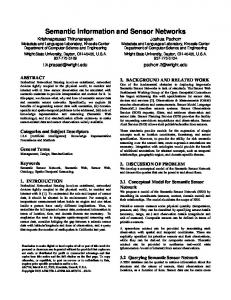
As we pointed out earlier, for a specific delivery zone, the more “compact” a network is, the smaller the forwarding zone needs to be. An immediate question is, can we design the sensor network so as to make its ∆-compactness value as close to the maximum value one as possible? As we want to continue with the random distribution assumption, there is only one design dimension left: the sensor node density. Note that we define sensor density as the average number of immediate network neighbors each node, rather than number of nodes in a unit area. Intuitively, the higher the sensor density, the “better” connected the sensor network is and the larger the corresponding network ∆-compactness is. To verify this observation, we designed the following experiment. We scatter 800 sensors uniformly distributed in a 1000x400 rectangular area, select only the configuration which is not partitioned at the range of 35. (Note because of random distribution, the network is sometimes partitioned.). Then we compute the values of ∆-compactness for the network formed by sensors assuming communication range value: 35 to 90. Note that in this experiment we choose to vary the communication range rather than to vary node density directly (by adding more nodes to the area). The reason we choose to vary the communication range as a mechanism to vary the relative sensor density is because this does not change the actual location configuration of the sensors in the experiment, and, in turn, makes the corresponding compactness value comparison more meaningful. The above procedure was repeated for five different configurations and the results (average values and standard deviations) are presented in Fig 10. Fig 10(a) shows the average (across the 5 runs) ∆-Dilation (defined as the inverse of ∆compactness ) versus the change of communication range. Fig 10(b) shows a corresponding figure with the average node degree as the x-axis. The results show that the network compactness indeed increases when the node density increase. But surprisingly, there appears to have a saturation point at a moderate density. The network exhibits a rapid increase in compactness (rapid decrease in ∆-dilation ) when the average number of
-
12
10
Area: 1000 X 400 Number of Nodes: 800 Spatial Dsitribution: uniform
Network Dilation
8
max dilation
6
4
2
max dilation of 99%
0 30
40
50
60 70 Communication Range (meters)
80
90
100
12
10
Area: 1000 X 400 Number of Nodes: 800 Spatial Dsitribution: uniform
Network Dilation
8 max dilation
6
4
2
0
max dilation of 99%
5
10
15
20
25 30 35 Average Number of Neighbors
40
(a)
45
50
55
(b)
Figure 10: (a)∆-Dilation vs Range, (b)∆-Dilation vs Average Number of Neighbors
neighbors changes from 8 to 15 and then starts to saturate. This appears to be an area to increase the compactness of the network with highest efficiency for these randomly distributed networks. This may provides a good heuristic for deploying mobicast/communication friendly sensor network. In addition, we also examined the value of the majorities of the pairwise ∆-compactness and how they change with node density. The lower curve in Fig 10(a) and (b) shows how the lower bound of the top 99% of the δ(i, j) of the network changes with node density. One can see that the occurrence of the lower extreme compactness value is a rare event. This further suggests that an optimistic choice of kcover for the forwarding zone is a good mobicast strategy in practice.
5. OPTIMISTIC MOBICAST To verify our observations about the potential benefit of optimistic mobicast on random networks with uniform distribution, we implemented an extended mobicast protocol on the ns-2 network simulator. Our implementation has a mode to let the user to specify the parameter (delta) for determining the forwarding zone. This allows us to test the trade-off between the message forwarding cost and the delivery guarantee. The header of our mobicast protocol packet contains the following information:
message type to delivery zone size (radius) sender packet sequence number delivery zone velocity (x and y components) sender location (x and y coordinates) delta factor sending time gamma factor message lifetime
Our protocol only provides support for a circular delivery zone. We also assume that the initial delivery zone is centered at the sender. One may augment the header with the information about the initial delivery zone center to allow applications to explicitly set the initial delivery zone location. Because this is not essential for our validation and verification test purposes, we simply default the sender location as the center of the initial delivery zone. Upon hearing a mobicast message m ˜ at time t. —————————— 1.if (m ˜ ) is new and t < T 2. cache this message 3. if the value of the delta field is zero 4. use local delta value for computation 5. else 6. use the value in the packet for computation 7. end if 8. if (I am in current forwarding zone F[t]) then 9. broadcast m ˜ immediately ; ¿ // fast forward 10. if (I am in current delivery zone Z[t]) then 11. deliver data D to the application; 12. else 13. compute my td [in]; 14. if td [in] exists and td [in] < T 15. schedule delivery of data D to the application layer at td [in]; 16. end if 17. end if 18. else 19. compute my tf [in]; 20. if tf [in] exists 21. if t0 ≤ tf [in] ≤ t 22. broadcast m ˜ immediately ; ¿ // catch-up! 23. else if t < tf [in] < T 24. schedule a broadcast of m ˜ at tf [in]; //hold and forward 25. end if 26. end if 27. end if 28. end if Figure 11: Optimistic Mobicast Protocol Our mobicast protocol is depicted in Fig 11. In this paper we omit the detail about geometric computation involved in determining if and when a node is in a forwarding zone and delivery zone, as it is not conceptually essential. Our mobicast protocol also maintains a transient message cache (it is periodically cleaned by throwing out expired messages). To minimize the dependence of simulation results on the network configuration used, our experiments were run on
five different connected network configurations generated via uniformly distributing 800 sensor nodes on a 1000x400m area. Fig 12 shows one such configuration example used. (Connectivity is not shown in this graph for clarity. Please see Fig 5 for connectivity. We used the exact the same distribution for the two graph in case the reader would like to compare.) One node close to the left is chosen as the mobi-
1
Delivery Ratio
0.8
0.6
0.4
0.2
0 0.5
1
1.5
2 2.5 Forwarding Zone Factor
3
3.5
4
3
Figure 12: Optimistic Mobicast Simulation Example Normalized Forwarding Overhead
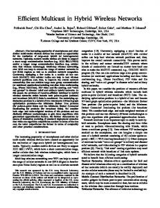
cast sender. Our results are averaged over multiple runs on five network configurations. For all runs, the delivery zone velocity is 40m/sec, from left to right, and each mobicast session has a lifetime of 20 seconds. For all the configurations used, the critical communication range for all the nodes to form a connected graph is between 30 to 35 meters. We chose the delivery zone radius to be 45 meters. We designed two sets of experiments. The first one intended to investigate how mobicast delivery ratio and forwarding overhead changes with the size of the forwarding zone on these uniformly distributed networks. Delivery ratio is defined as the percentage of delivery-zone nodes (those that are in the virtual delivery zone at some point of time during a mobicast session) that actually received the mobicast message. Forwarding overhead is defined as the number of extra message transmissions per node delivery, i.e, the total number of retransmissions minus and then divided by the number of delivery zone nodes that actually received the message. Fig 13(a) shows the simulation results of delivery ratio versus the forwarding zone factor (the actual k used in forwarding zone computation. One may view it as the inverse of the sender’s view about the network’s compactness.). The high variance in the value is due to random distribution of holes across different configurations, which causes each mobicast session to stop prematurely at different locations across at different configurations. The limited number of network configurations used also contribute to this. Fig 13(b) shows how the forwarding overhead changes with the forwarding zone factor. The second set of experiments were designed to investigate how the delivery ratio is affected when the network becomes more compact. Due to the limited scalability of ns2, we again change of the communication range to change compactness, rather than by adding more nodes. In the experiment, the delivery zone radius used is 45 meters. The communication radius varies from 35 to 45 meters. We collected results from multiple runs of mobicast using different forwarding zone factors over the five configurations and results are summarized in Table 1. From the results we can see that indeed the delivery ratio increases when node density increase. Again the high variance in the value is due to random distribution of holes across different configurations and each mobicast session stops prematurely at different locations across at different
2.5
2
1.5
1
0.5
0 0.5
(a)
1
1.5
2 Forwarding Zone Factor
2.5
3
3.5
(b)
Figure 13: (a) Delivery ratio vs Forwarding Zone Size; (b) Normalized Forwarding Overhead vs Forwarding Zone Factor configurations. In our simulation, we also examined the timeliness of mobicast delivery on these networks. More specifically, we would like to see how far ahead a node received the mobicast message before entering the delivery zone (or how late after entering the delivery zone). Fig 14 shows one typical result of a mobicast session, when the communication range is 35m, the delivery zone radius is 45m, δ is 0.7, and the mobicast speed is 40m/s. Fig 14 shows the mobicast packet reception time relative to the sending time, for all the nodes that were ever in the delivery zone. The solid line is the expected reception deadline for nodes in each location, i.e, the first time they are expected to enter the delivery zone. The star dotted line is the actual reception time of the mobicast packet for each node. For comparison, we also included a simulation result (the diamond dotted line) of a spatial multicast on the same path with “as soon as possible” delivery (Note that in this case the spatial propagation speed exceeds 1600m/s, 800m traversed in less than half second). We can clearly see the temporal locality property of mobicast. The packet reception time is very close to the deadline specified by the delivery zone semantics. These result also suggests the benefit of mobicast over a more conventional spatial multicast like geocast, which assumes implicit assoon-as-possible temporal delivery semantics, i.e, using mobicast one can control to information propagation speed to
Table 1: Effects of Delivery Zone Size and Forwarding Zone Factor on Delivery Ratio R\δ 1.0 0.9 0.8 0.7 0.6 0.5 0.4 0.3 35 0.69± 0.29 0.78± 0.29 0.80± 0.28 0.90± 0.21 0.90± 0.21 0.99± 0.10 1 1 40 0.90± 0.21 0.90± 0.21 0.90± 0.21 1 1 1 1 1 45 0.998± 0.003 1 1 1 1 1 1 1
pactness also appears to be uniformly distributed spatially. This suggests that in such networks, local adaptation may not provide significant improvement for mobicast with respect to its efficiency. For networks that have distinct and
20 18
Delivery deadline Mobicast velocity: 40m/s ASAP Spatial Multicast
16 14
1
Reception Time
12
0.9
10 8
0.8
6
0.7 Average local delta
4 2 0 S −2
0
100
200
300
400 500 600 Location of Nodes
700
800
900
1000
0.6 0.5 0.4 0.3 0.2
Figure 14: Slack Time of Mobicast Delivery
0.1 0
better satisfy application needs while without making spatiotemporally unrelated nodes unnecessarily busy. We believe this “just-in-time” delivery capability of mobicast is a powerful mechanism for resource utilization optimization for related applications in sensor network.
0
100
200
300
400
500 X Location
600
700
800
900
1000
0
100
200
300
400
500 X location
600
700
800
900
1000
1 0.9 0.8
6. ADAPTIVE MOBICAST So far we have discussed two ways to improve mobicast in uniformly distributed sensor networks: (1) Making the network more compact by choosing an optimal node density; (2) Using an optimistic choice for the forwarding zone size by slightly relaxing the delivery guarantee. A third mechanism likely to improve mobicast is to let the protocol adapt to a local notion of compactness. For instance, when the mobicast delivery zone moves from a more compact area into a less compact one, its forwarding zone will expand. If the delivery zone moves from a less compact area into a more compact one, its forwarding zone should shrink. The local notion of compactness can be area-based or per-node based. For instance, one may partition the space into a grid and compute the compactness value for each grid area. Or one may let each node probe up to certain depth into its neighborhood and compute the compactness around it. The latter is what we use in our adaptive mobicast simulation (presented next). This type of local compactness adaptation is beneficial when the network is indeed more compact in one area and less so in others and the difference in compactness is relatively large. Yet, our preliminary investigation shows that for random networks with uniformly distribution, all areas have similar compactness. Fig 15 shows one example of the spatial distribution of local compactness for a uniformly distributed network of size 1000x400 (as the one in Fig 5). The local compactness is computed for each node to a depth of five hops and within a 100 meter radius. One can see that for uniformly distributed networks, local com-
Distribution of local delta
0.7 0.6 0.5 0.4 0.3 0.2 0.1 0
Figure 15: Local Delta Distribution Over Space (Uniform Distribution) relatively long range spatial variations in compactness, we expect adaptive protocols to excel. In order to verify the above observations, we modified the previous mobicast (Fig 11) and made it adaptive in the following manner. First, the header is augmented with an extra field: location (x,y), which is used for recording the location of the most recent delivery-zone node that handled the packet. In the adaptive mobicast protocol, when receiving a packet, a delivery zone node will replace the delta value in the packet by its local delta value before forwarding it. This is an attempt to inform other downstream nodes about its view of the network compactness. A node finding itself not to be a delivery-zone node upon receiving a mobicast packet will use the delta in the packet to determine its own forwarding status (forward immediately, schedule for future forward, or drop the packet). If a non-delivery-zone
1 0.9 0.8
Average local delta
0.7 0.6 0.5 0.4 0.3 0.2 0.1 0
0
100
200
300
400
500 X Location
600
700
800
900
1000
0
100
200
300
400
500 X location
600
700
800
900
1000
1 0.9 0.8 0.7 Distribution of local delta
node finds that it is a forwarding-zone node, it forwards the packet but does not make any change to the delta value in the packet. The reason for this forwarding behavior difference between delivery-zone nodes and non-delivery-zone nodes is that the purpose of forwarding is to guarantee the mobicast delivery for the delivery zone nodes. The potential path distortion between delivery zone nodes is expected be be captured by the local compactness values of the delivery zone nodes. Depending on the network topology, there are cases where a forwarding node is relatively far away from the delivery zone, so having a very different neighbor topology, and by replacing the delta with its own, downstream nodes might be mis-informed. Our preliminary simulation results of this adaptive mobicast protocol in ns-2 is as follows. For the uniformly distributed network topology such as the one in Fig 5 and Fig 12, the adaptive protocol appears to guarantee 100% delivery4 , but the delivery overhead is about two radio transmissions per delivery, which is relatively high. The reason is, as we pointed out earlier, that holes are ubiquitous in the random network and most of the nodes have some worst form of path distortion in their neighborhood. And the collective behavior of the protocol forms a forwarding zone whose size in determined by the smallest compactness in each subarea. In turn caused more nodes to participate in the forwarding. To examine the behavior of our adaptive mobicast protocol in more detail, we hand-crafted a well-connected network in a 1000x400 area with 800 nodes, with with a big hole at the center, as shown in the top side of Fig 16. For this topology, the compactness value for the nodes close to the hole is distinctively smaller than the nodes close to both ends, as shown in Fig 17. The bottom picture of Fig 16 shows
0.6 0.5 0.4 0.3 0.2 0.1 0
Figure 17: Local Delta Distribution Over Space on its path. The radio transmission overhead is less than 1.2 transmissions per delivery in the above case (195 extra radio transmissions for 164 delivery zone node deliveries).
7.
Figure 16: Example of Adaptive Mobicast a mobicast session run from a node on the left to the right. The delivery zone has a radius of 45, and moves at a speed of 40 m/s with a session length of 20 seconds. The circled nodes are those participated in the mobicast session. One can see that the protocol adapts to the local topology, and achieves 100% delivery, even in the presence of a big hole 4 Note that we only experimented on a limited number of configurations, this 100% is not equivalent to an absolute guarantee. Actually, in theory, sometimes this adaptive protocol will not have 100% delivery, because the local compactness value only captures the topology distortion in a limited scope.
DISCUSSION
An important aspect of mobicast is that applications have control over the velocity of information dissemination over the space. This brings many new spatial and temporal coordination and interaction possibilities across a network. For instance, an application might use a mobicast to send some information to the east at a speed of 40 miles per hour. One second later, it may find an error in that information, for instance, there is a change in the intruder’s expected path, and want to send the new information and stop further propagation of the old information on the network. Note that stopping previous information dissemination is impossible in conventional protocols which have explicit or implicit “assoon-as-possible” delivery semantics. Yet, in mobicast, a “stop that message” message can be sent at a much higher speed, say 120 miles per hour, (or even more than 1000 miles per hour which we found possible in our simulation), with a same-size delivery zone along the previous path. Clearly, this new mobicast recall message can easily catch up with its target message which propagates at a much lower speed. As spatiotemporal protocols are relatively new, there are many research questions waiting to be answered. For instance, our ns-2 simulations are run without background traffic. When there is background traffic, the one-hop la-
tency will change and will have a higher variance. Also, more collisions will happen and more packets will be lost. We know that theoretically the temporal guarantee is based on the assumption of the worst-case one-hop communication latency τ1 . The estimation of τ1 in practice should consider the anticipated competing traffic. We note that modelling communication delay at the MAC layer is an active research area, but is out of the scope this paper so we do not address it here. Note also that there is a tradeoff between the just-in-time delivery property and the guarantee on the delivery deadlines. A conservative estimation on τ1 may guarantee the delivery before deadline but might lead to many too-early deliveries. Nevertheless, how exactly the background traffic will affect the delivery ratio and timeliness of the spatiotemporal protocols and how the protocols shall be adjusted accordingly, how different traffic patterns and data sending rate may effect the protocols, are among the questions we seek to answer in the near future. Furthermore, location information are used in computing the compactness values. Imprecise location information will introduce error in the compactness value. Our investigation in the effect of node density on the compactness values and optimistic mobicast a first step in addressing the question about the effect of imprecise location information (note that only the density is the true variable in the study). Deeper investigation on the issue of imprecise information should provide us more insight into the problem. For simplicity of presentation, our protocol essentially carries out flooding inside the forwarding zone. If the nodes have an accurate picture about the locations of their one-hop or two-hop neighbors, then one can reduce the number of necessary re-transmissions by using this knowledge in a manner similar to techniques proposed for improving broadcast efficiency [20, 21]. In a probabilistic guarantee scenario, one may also use probabilistic retransmission-reduction techniques such as the one proposed in [19]. A review of these and other related methods can be found in [23]. Our protocol, by only using the compactness values of the network, tries to used minimum number of bits to capture relevant topologies for spatiotemporal protocols. If the nodes assume for local knowledge about the network topology about its neighborhood, for instance, know the locations of all nodes within certain distance, more communication efficient mobicast protocols can be designed (while can be more computation intensive). Note that our protocols are routing layer protocols and we are only concerned about the routing layer overhead. The only function of the MAC layer they use is the MAC layer broadcast. Different MAC layer implementation and tuning may result in different MAC layer control overhead. However this is not a theme of our paper so we omit it. Finally, while the mobicast protocol we presented applies to the cases where the delivery zone moves through the space at constant velocity ~v for a duration T , mobicast in general applies to a much wider set of spatiotemporal constraints. The delivery zone can exhibit any evolving characteristics as long as it is sustainable by the underlying system. While they may all require similar ideas of forwarding zone and headway distance to maintain the spatiotemporal properties inherent in mobicast, different types of delivery zones may require different protocol handling details. Classification of a useful set of mobicast delivery zone scenarios and the design of the corresponding mobicast protocols are also
important elements in our future work.
8.
RELATED WORK
Mobicast is motivated by the need for coordination activities related to moving entities in the physical environment. In [4], Cerpa et. al. proposed a Frisbee model in an active sensing zone move through the network along with the target. [14] and [5] proposed data service protocols for improving the accuracy of distributed sensing in mobile environments. Both protocols entail communication schemes that push information about the object to the nodes close the projected location of the object in the future. The EnviroTrack group management protocol [1] dynamically creates and maintains a group that tracks mobile entities in the environment. However, neither of the aforementioned projects include communication mechanisms geared toward meeting explicit spatiotemporal constraints related to mobility. Mobicast can be viewed as complimentary to these projects by providing a convenient underlying communication mechanism that allows applications to push information with specific specified spatiotemporal requirements. The idea of disseminating information to nodes in a geographic area is not new. Navas and Imielinski proposed geographic multicast addressing and routing [10, 18], dubbed “geocast,” for the Internet. They argued that geocast was a more natural and economic alternative for building geographic service applications than the conventional IP addressbased multicast addressing and routing. In a geocast protocol, the multicast group members are determined by their physical locations. The initiator of a geocast specifies an area for a message to be delivered, and the geocast protocol tries to deliver the message only to the nodes in that area. Ko and Vaidya investigated the problem of geocast in mobile ad hoc networks [13] and proposed to use a “forwarding zone” to decrease delivery overhead of geocast packets. Other mechanisms [22, 15, 2] have been proposed to improve geocast efficiency and delivery accuracy in mobile ad hoc networks. Zhou and Singh proposed a content-based multicast [24] in which sensor event information is delivered to nodes in some geographic area that is determined by the velocity and type of the detected events. While different in style and approach, all these techniques assume the delivery zone to be fixed. They also assume the same information delivery semantics along the temporal domain, i.e., information is to be delivered “as soon as possible”. However, local coordination often requires just-in-time delivery in sensor networks. Data aggregation is an important information processing step in sensor networks. Several techniques have been proposed to support data aggregation in sensor networks. For example, both directed diffusion [12, 11] and TAG [16] allow data to be aggregated on their route from the sources to a base station. No explicit local coordination is supported by these techniques. LEACH [7] organizes sensors into local clusters where each cluster head is responsible for aggregating the data from the whole cluster. However, there is no notion of mobility and the clusters do not move in space following a physical entity. In contrast, supporting local coordination for mobile physical entities is a primary goal of mobicast.
9.
CONCLUSION
Mobicast is a novel spatiotemporal multicast protocol that distributes a message to nodes in a delivery zone that evolves over time in some predictable manner. The key advantage of mobicast lies in its ability to provide reliable and justin-time message delivery to mobile delivery zones on top of a random network topology and spatial distribution. Our mobicast protocol seeks to used minimum amount of information about network topology, i.e., the compactness of the network, to achieve a reliable spatiotemporal information delivery. In this paper, we first investigated network compactness properties which are relevant to spatiotemporal propagation, on uniformly distributed networks. We found the distribution of values for the compactness metric in randomly distributed sensor networks to be highly concentrated around a peak close to one with a very small portion close to zero. This leads to the identification of a fundamental tradeoff between probabilistic delivery guarantees and communication overhead in spatiotemporal multicast. We found that mobicast can significantly reduce its communication overhead via a propitious choice of forwarding zone size by only a slight relaxation of its delivery guarantee. We also designed an adaptive mobicast protocol which exhibits promising delivery behaviors in simulation. We also investigated the impact of node density on network compactness. We found that the network compactness improves as the node density increases, and surprisingly this behavior saturates at a medium level density. This suggests the existence of an optimal node density for supporting mobicast over a randomly distributed sensor network. We hope this work will help to facilitate a broader research effort in spatiotemporal communication mechanisms and sensor network applications.
10. REFERENCES [1] B. Blum, P. Nagaraddi, A. Wood, T. Abdelzaher, S. Son, and J. Stankovic. An entity maintenance and connection service for sensor networks. The First International Conference on Mobile Systems, Applications, and Services (MobiSys), San Francisco, CA, May 2003. [2] J. Boleng, T. Camp, and V. Tolety. Mesh-based geocast routing protocols in an ad hoc network. In Proceedings of the IPDPS in Wireless Networks and Mobile Computing, pages 184–193, April 2001. [3] P. Bose, L. Devroye, W. Evans, and D. Kirkpatrick. the spanning ratio of gabriel graphs and -skeletons, 2001. [4] A. Cerpa, J. Elson, D. Estrin, L. Girod, M. Hamilton, and J. Zhao. Habitat monitoring: Application driver for wireless communications technology. In ACM SIGCOMM Workshop on Data Communications in Latin America and the Caribbean, Costa Rica, April 2001, 2001. [5] M. Chu, H. Haussecker, and F. Zhao. Scalable information-driven sensor querying and routing for ad hoc heterogeneous sensor networks. Int’l J. High Performance Computing Applications, 2002. [6] D. Eppstein. Spanning trees and spanners. In In J.-R. Sack and J. Urrutia, editors, Handbook of Computational Geometry, pages 425–461, Amsterdam, 1999. Elsevier Science.
[7] W. R. Heinzelman, A. Chandrakasan, and H. Balakrishnan. Energy-efficient communication protocol for wireless microsensor networks. In HICSS, 2000. [8] Q. Huang. Spatiotemporal Multicast and Partitionable Group Membership Serivce. PhD thesis, Washington University, St. Louis, August 2003. [9] Q. Huang, C. Lu, and G.-C. Roman. Mobicast: Just-in-time multicast for sensor networks under spatiotemporal constraints. In IPSN’03, 2003. [10] T. Imielinski and J. C. Navas. Gps-based addressing and routing. RFC2009, Computer Sciece, Rutgers University, March 1996. [11] C. Intanagonwiwat, D. Estrin, R. Govindan, and J. Heidemann. Impact of network density on data aggregation in wireless sensor networks. Proceedings of the ICDCS-22), 2001. [12] C. Intanagonwiwat, R. Govindan, and D. Estrin. Directed diffusion: a scalable and robust communication paradigm for sensor networks. In Mobile Computing and Networking, pages 56–67, 2000. [13] Y. Ko and N. Vaidya. Geocasting in mobile ad hoc networks: Location-based multicast algorithms, 1998. [14] D. Li, K. Wong, Y. Hu, and A. Sayeed. Detection, classification and tracking of targets in distributed sensor networks. IEEE Signal Processing Magazine, 19(2), March 2002. [15] W.-H. Liao, Y.-C. Tseng, K.-L. Lo, and J.-P. Sheu. Geogrid: A geocasting protocol for mobile ad hoc networks based on grid. Journal of Internet Technology, 1(2):23–32, 2000. [16] S. Madden, M. Franklin, J. Hellerstein, and W. Hong. Tag: a tiny aggregation service for ad-hoc sensor networks. OSDI 2002, Boston MA. [17] G. Narasimhan and M. H. M. Smid. Approximating the stretch factor of euclidean graphs. SIAM J. Comput., 30(3):978–989, 2000. [18] J. C. Navas and T. Imielinski. Geocast - geographic addressing and routing. In Proceedings of MobiCom ’97, pages 66–76, 1997. [19] S.-Y. Ni, Y.-C. Tseng, Y.-S. Chen, and J.-P. Sheu. The broadcast storm problem in a mobile ad hoc network. In Proceedings of the MobiCom’99, pages 152–162, August 1999. [20] W. Peng and X. Lu. On the reduction of broadcast redundancy in mobile ad hoc networks. In Proceedings of the ACM Symposium on Mobile Ad Hoc Networking and Computing (MOBIHOC), 2000. [21] A. Qayyum, L. Viennot, and A. Laouiti. Multipoint relaying: An efficient technique for flooding in mobile wireless networks. Technical Report Research Report RR-3898, INRIA, Feb. 2000. [22] I. Stojmenovic. Voronoi diagram and convex hull based geocasting and routing in wireless networks. TR TR-99-11, University of Ottawa, December 1999. [23] B. Williams and T. Camp. Comparison of broadcasting techniques for mobile ad hoc networks. In Proceedings of the ACM MOBIHOC’02, pages 194–205, 2002. [24] H. Zhou and S. Singh. Content based multicast (cbm) for ad hoc networks. MOBIHOC, August 2000.